Building an Electric Racing Motorbike from Scratch
Introduction
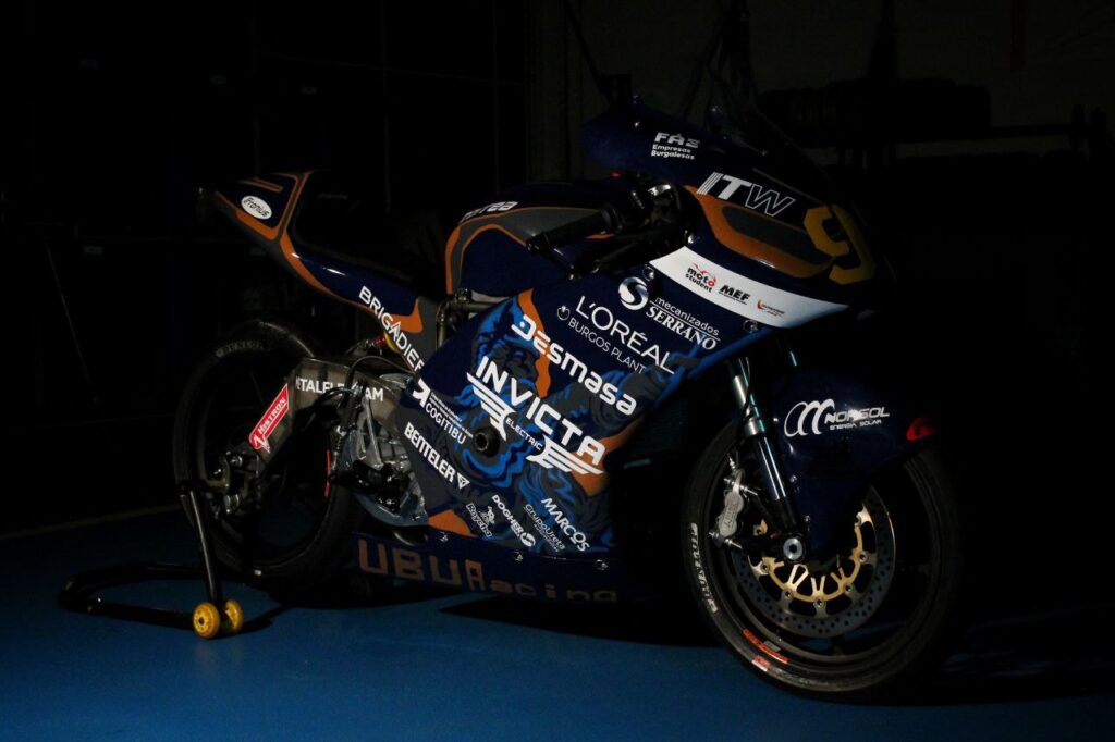
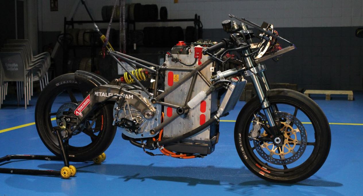
Motostudent is an international competition where students must design, build, and test a prototype racing motorcycle. In this post, I will summarize around a year of work and walk you through the process of building an electric racing motorcycle from scratch. This project covers a wide range of technical and non-technical areas, which I will break down into key sections. The main sections will focus on mechanical, electrical, and powertrain aspects, each of which includes numerous subsections as outlined in the index.
Approach to the Project
As told before, the goal of the project is to design and build an electric motorbike. The main aim should be to apply all this knowledge, that we were supposed to have learned in the university, into a practical real world scenario.
We were racing in representation of the University of Burgos (which didn’t help too much to the team). We didn’t even have a space for work inside the university, so we looked for local companies that allowed us to work at their facilities and with their tools, machines etc. I left the university a few years ago, but I enrolled in one subject again to participate in this project (Motostudent organization requires team members to be enrolled in the university to participate in the final event). The project is supposed to be extended during two years, but the real execution of the project always is less than that. All the work shown here has been made in 8 months (plus some experience from the previous edition).
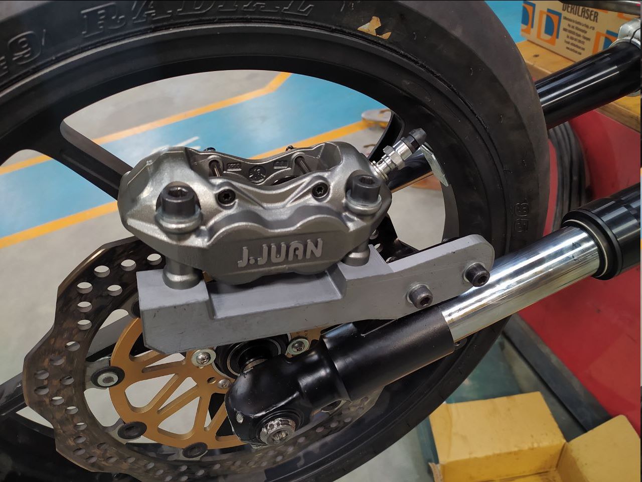
In Motostudent, we can find two categories: petrol and electric. In both categories, the organization gives you a pair of tires, front and rear brake calipers and front and rear brake pumps. In the petrol category they give you a 250cc 4-stroke KTM engine. In the electric one, they give you a 3-phase permanent magnet AC electric motor and IMD (Insulation Monitoring Device, we will talk about it later). We will talk about the motor later too.
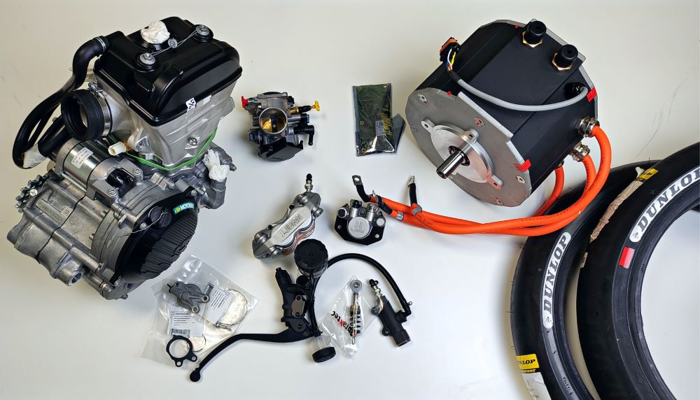 Material provided by the organization in the 2022-2023 edition.1
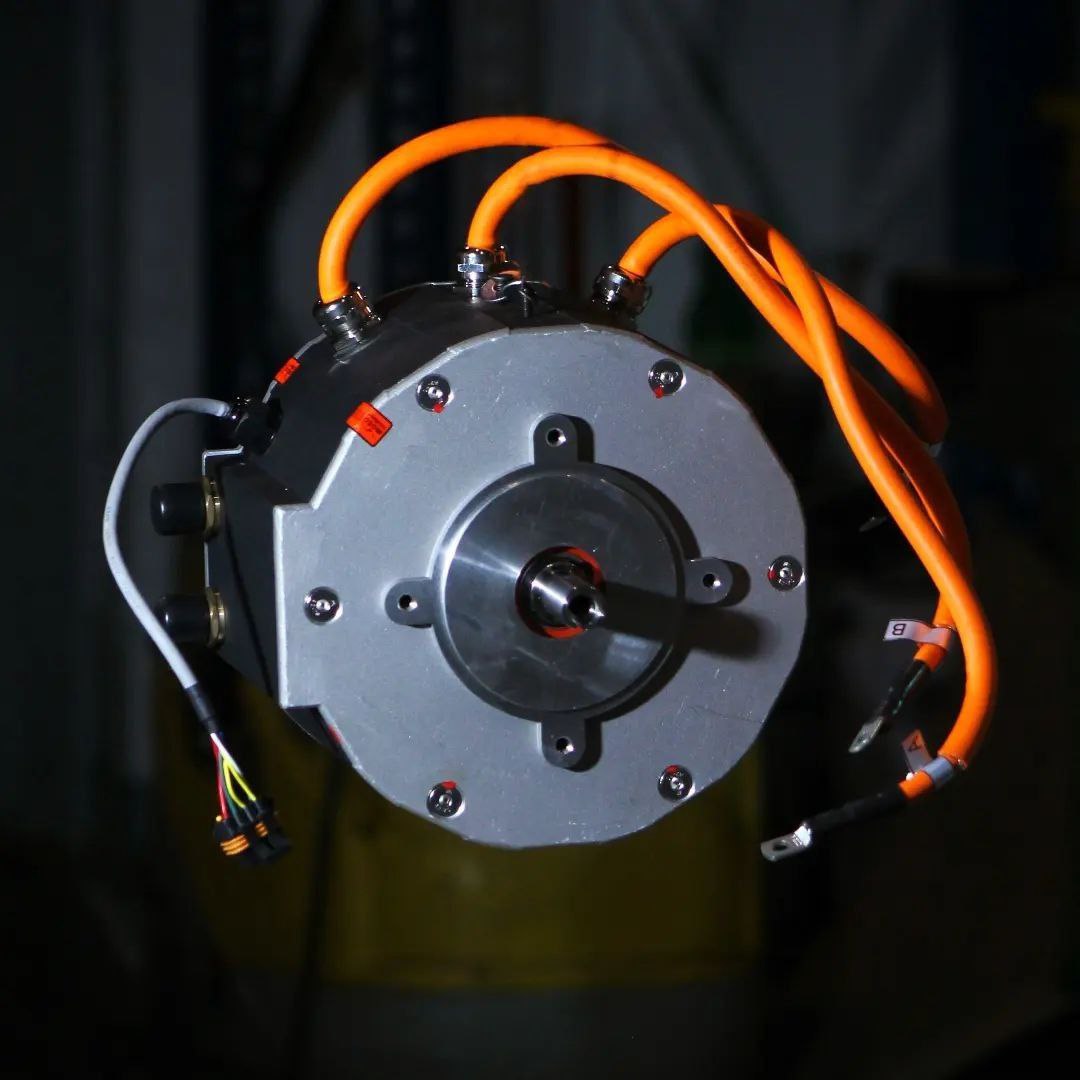 Liquid-cooled electric motor Liquid-cooled electric motor |
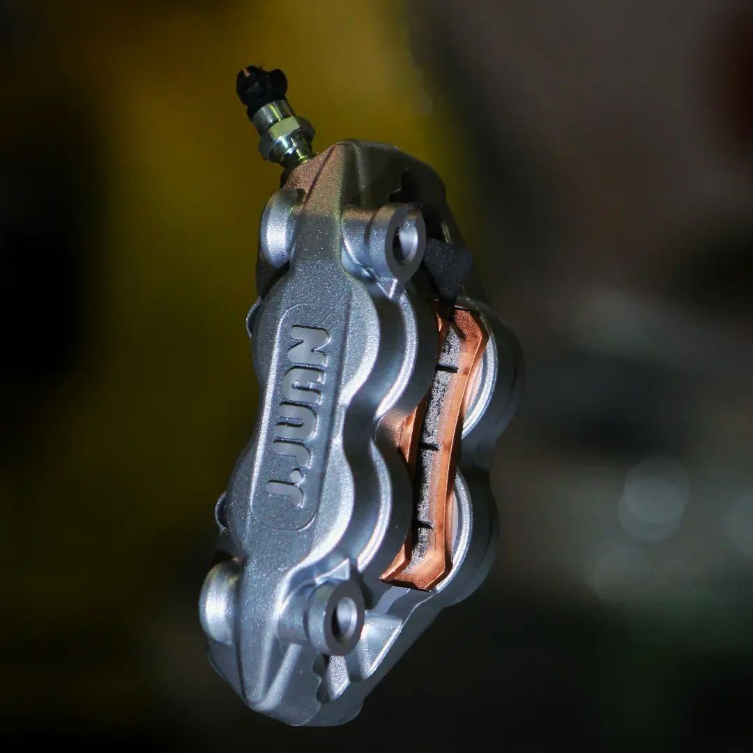 JJUAN front brake caliper JJUAN front brake caliper |
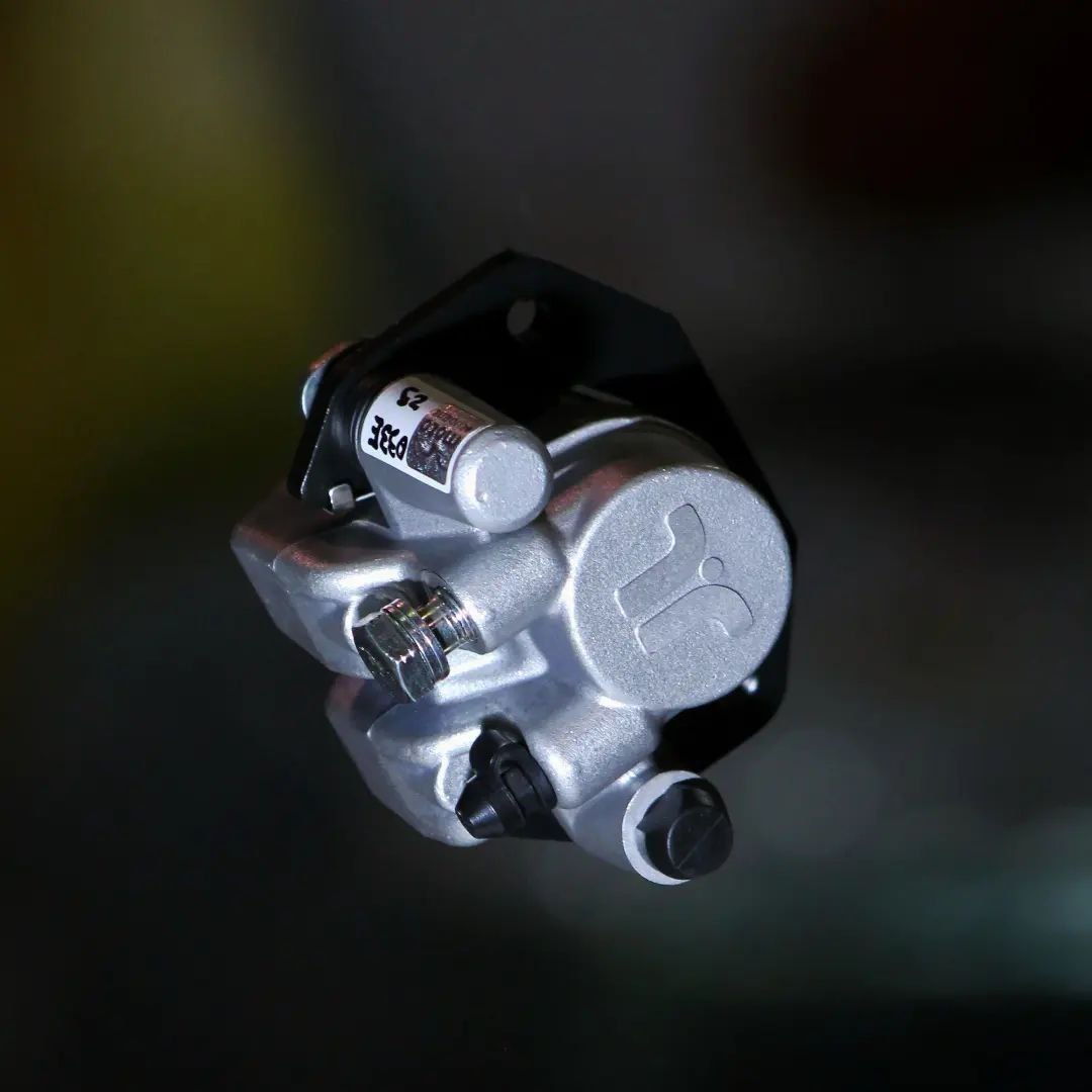 JJUAN rear brake caliper JJUAN rear brake caliper |
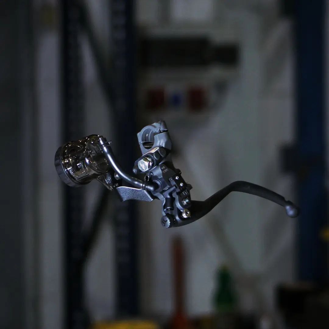 JJUAN front brake pump JJUAN front brake pump |
 Dunlop Moto3 tyres Dunlop Moto3 tyres |
The team must send some documentation to the organization for evaluation and to check if, for example, minimum safety measures are accomplished, such as battery assembly, structural rigidity, etc.
Once the prototype is finished, there is a final test at the Motorland circuit, in Aragon, Spain. All the teams travel one week with the prototypes to race against others.
 Motostudent final event1
There are two types of tests on the final event:
Static tests: In these tests, the organization verifies whether the prototype meets safety standards and regulations.
- Weight check: There is a minimum weight on the prototype of 85 kg, but in the electric category we are far away from that weight.
- Load check: The organization loads 250 kg on the seat and 300kg between axles and checks the structural behavior of the prototype.
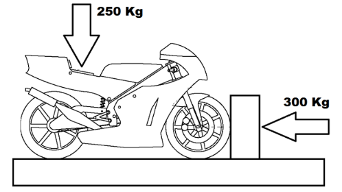 Illustration on regulations about static test |
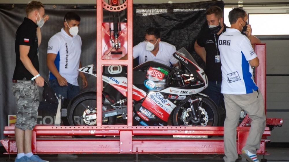 Static test of a Polish team's prototype |
- Brake check: The Organization tests the brakes of the prototype with a dynamo-meter.
- Isolation resistance measurement check: The isolation between the high voltage and the prototype chassis must be at least 100 ohms/V.
- IMD check: Organization connects a 50k ohm resistor between the chassis and battery positive. The IMD must open the circuit and cut the power (HV) in 30 seconds. Our prototype cut in 2 seconds.
- Rain check: Organization sprays water during 60 seconds and waits another 60 seconds. The prototype must work after that time, simulating rain conditions.
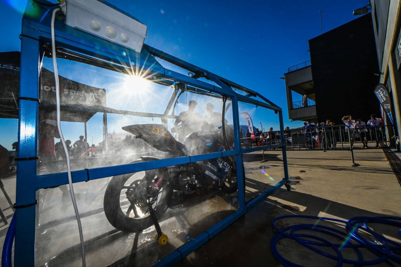 Rain test of the current prototype1
Dynamic tests: In these tests the teams compete against each other to see which is the best in each category.
- Brake test: The prototype must enter at 80km/h and brake as soon as possible. The shortest distance wins.
 Braking test1
- Gymkhana: There is a small circuit and they test the maneuverability of the bike. A good rider is important here!
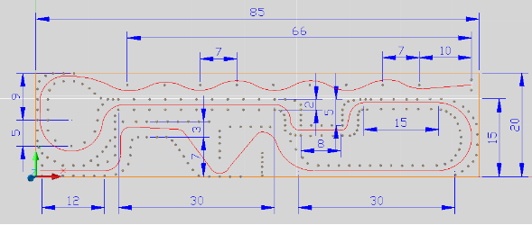 Sketch of the gymkhana1
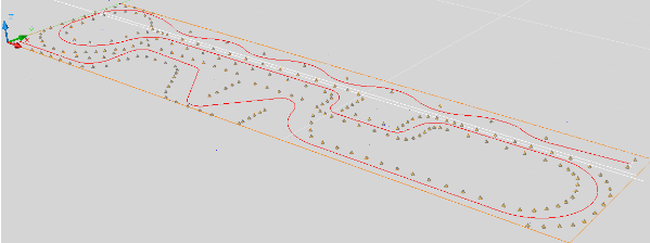 3D Sketch of the gymkhana1
- Acceleration: Organization checks the time spent to accelerate from 0 to 150 meters.
- Max speed: Maximum speed is checked at the end of the rear straight.
- Regularity: One sector of the circuit is measured during multiple laps to check how regularly the teams can do the sector, trying to make the same time on all laps.
- Pole position: Fastest prototype in one lap.
- Best race lap: Fastest lap of a prototype in the race.
- Race: Final race between all teams. It’s 6 laps to Motorland MotoGP Circuit with 5 km per lap that give us around 30 km of race.
Previous Editions
I gave a short introduction about the competition and some of its regulations. That’s everything we had when we started the project, nothing more. We didn’t even have a euro to start or a place to work. The team was very small, it’s difficult to find people with commitment nowadays and more on a project like this that requires too much time and effort and doesn’t give any salary or short-term rewards.
Motostudent has an edition every two years. The University of Burgos has been participating during the previous 6 editions. All of these editions with petrol bikes except the last one and the third year that they did both, petrol and electric. From my point of view, there are some big problems with the team:
- The team is renewed every edition: In all previous editions, there weren’t people from the previous edition, so there is no relief.
- Lack of university involvement: It’s assumed that the team represents the university, but there aren’t even teachers following the project. There is also no place to meet and store all the things and materials of the project. The university doesn’t even pay for the full registration of the team!
- There is no documentation: There is no more documentation than the reports sent to the organization on previous editions and that doesn’t cover everything or important aspects of the technical challenges solved in previous editions.
- There was no knowledge: The first electric prototype was started (from the electrical point of view) not by the students. They were helped by an external company, so no internal knowledge could be left on the team.
- Decline in education: Getting a degree nowadays is easier than ever. Students leave the university without the minimum knowledge and foundation about the degree they are studying at the level that an electronic engineer student on their last year doesn’t know the difference between series and parallel connections. Imagine if you have to build an electric motorbike or a battery with that knowledge! You need to re-teach students again only for the project.
I joined the team late on the second electric prototype (2020-2021). Of course, I didn’t have any idea about how to program the inverter, how batteries work, or even some basic electrical concepts (I’m computer engineer). That’s what I will try to explain in all these posts and keep a documented record of the process.
I will focus on the actual prototype as in the previous one there were a lot of decisions taken when I arrived, but let’s look at it briefly.
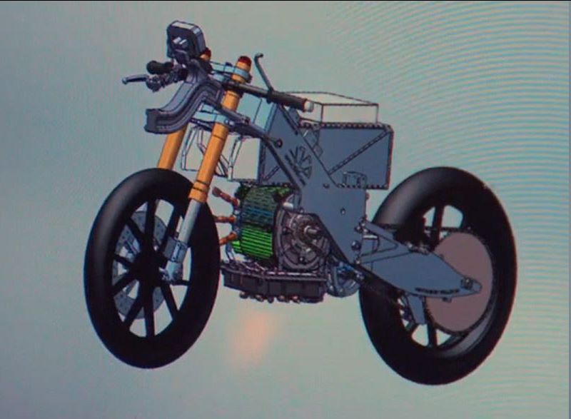
Here is a CAD of the previous prototype:
 Unfinished 3D design from previous prototype.
The 3D design wasn’t even finished and a lot of things were done on the fly. I don’t like that methodology because CAD software exist for something. When something is not designed and it’s manufactured in a hurry, it is a mess (laser cutting vs rotaflex for example).
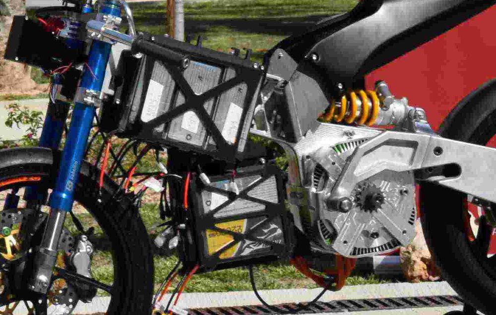
One of the many decisions that were done without a reason (or knowledge) was the battery package. This prototype had a Brutepower cells. The decision was taken because other teams had it on previous editions. These cells were Chinese 22.000 mAh cells of LiPo technology. They were mounted in a 24s 4p configuration. This means, 24 cells in series and 4 cells in parallel, giving a 88Ah and 100.8V on full charge. As we will see on battery section, this was a wrong decision as these cells are not suitable for this use.
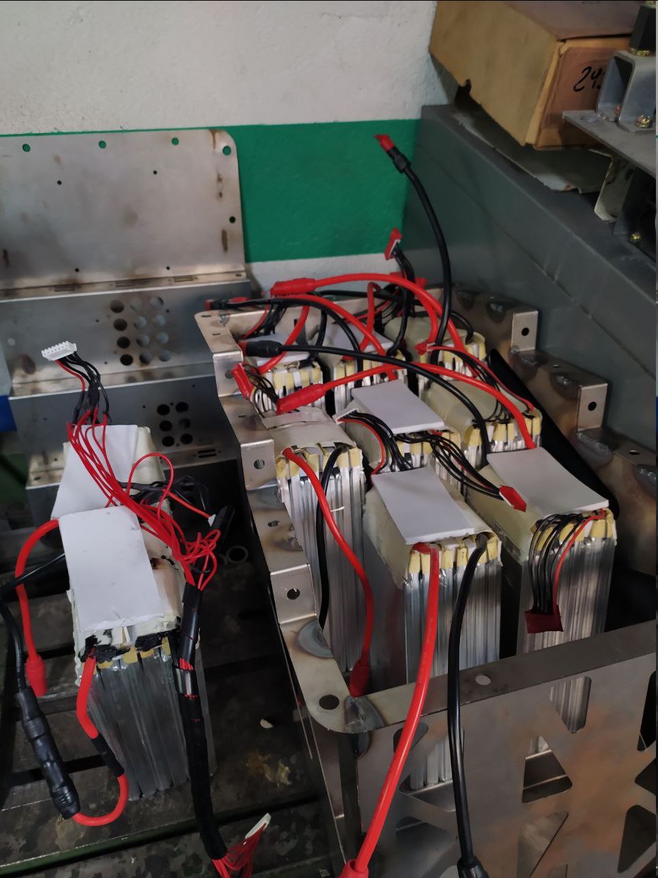 Previous prototype battery chaos |
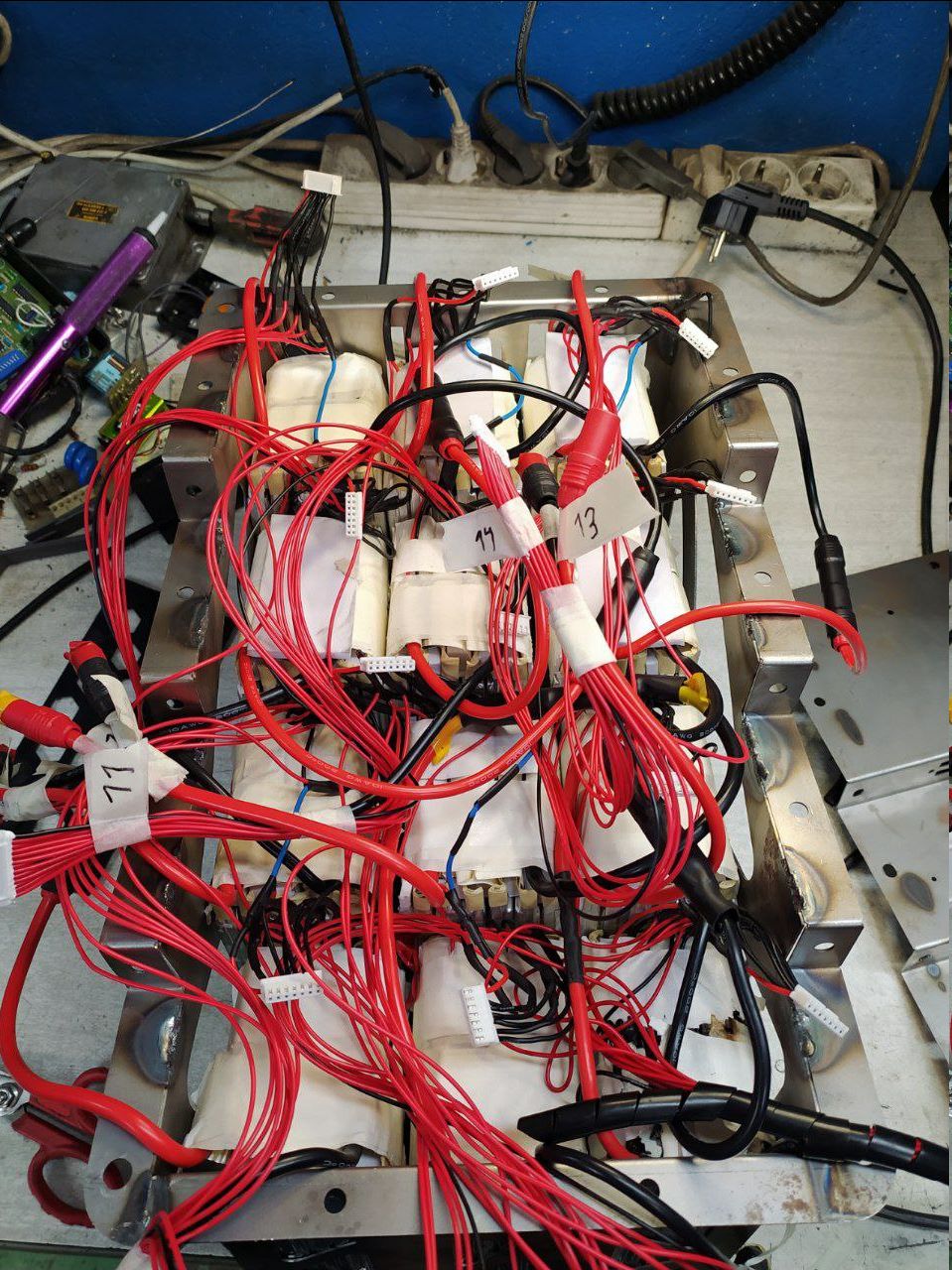 Previous prototype battery connections and wires |
And of course, on that edition, inverter programming was stock. The organization of Motostudent sent us a programmed file (DCF) which wasn’t working correctly so the inverter was turning off repeatedly (overcurrent error).
Actual Prototype
Finishing the previous edition I realized what a great contribution and opportunity this project could be for me. The material and resources we can access are something very expensive that would be almost impossible to do privately. This motivated me to take the reins of the project for this edition. As mentioned before, we started with no money so our first approach was to take some sponsors. I will speak about this shortly.
Sponsorship
We needed to sell something, a brand, a product, an idea. To do this we needed to have a portfolio to present ourselves to companies and obtain sponsorship. We begin by creating all the necessary material:
- Web page (www.uburacing.es)
- Portfolio
- Sponsorship levels
- Slides
- All documents necessary for showing the project.
The first thing everyone thinks is that we could have sponsors in exchange of visibility. We put a sticker on the bike and they give us money or resources to accomplish the project. The reality is that a project like this does not have the visibility that it should, so we looked for other alternatives.
Nowadays companies are very “committed” to society (Agenda 2030, SDG, etc.), so we tried to generate a discourse that was related to that. Burgos is a city with a lot of industry and it is also true that many people who have finished their studies leave the city, so we had the discourse we needed there (keep talent here).
 Our main idea was “the talent of young people”. In a small city like Burgos, companies need skilled workers. This is the perfect project for people with special interest in the technical field beyond university studies. In exchange, companies that support the project could get this skilled people to work with them.
Companies need to support this project to train emerging talent and prevent young people from leaving the city, as well as make their companies known between this young students. This is also something socially responsible for companies. We, in return, would deliver the resumes of the team members (although unfortunately we didn’t have many).
With everything ready, we started to contact everyone we could through email, phone, meetings, etc.
One thing that worked very well for us was to going to events where owners / CEOs met. We were lucky to be able to show the project to this profiles on two “private” big events in the city. In addition, there, we could make direct contact with them and close a meeting to explain the project to them in more detail later. On the other hand, if they liked it, they could recommend us to owners from other companies.
Mainly, we had 2 types of sponsorship, economical and manufacturing. The companies that could manufacture something helped us with that (sheet metal, machining, materials), and the companies that couldn’t, helped us in the economical way (money).
Thankfully, we got all the budget, support and materials necessary to accomplish the project (around 30.000€), but not with too much time to finish it, so we started working in parallel on the technical field.
Someone will think, 30.000€ for an electric motorbike? Yes, because it’s not only the motorbike. We need parts for testing, spare parts, different sprockets and chains to play with, chargers for the batteries and also we needed to pay the administrative services for the association and, of course, taxes! And this budget is only for material, not including our working hours.
Technical Challenges
The main challenge was that we didn’t have any idea about how to accomplish a project like this, so we started step by step.
The areas into which we divided the technical challenges were:
- Mechanical
- Chassis and swingarm design
- Fairing
- Electronics
- Electrical circuit
- Telemetry
- Powertrain
- Battery pack design and manufacturing
- Inverter programming
Each of these categories are composed by much more specific categories that we will dissect below.
Mechanical ⚙️
Dyno
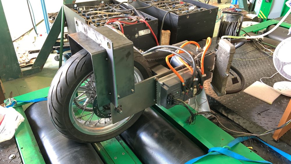
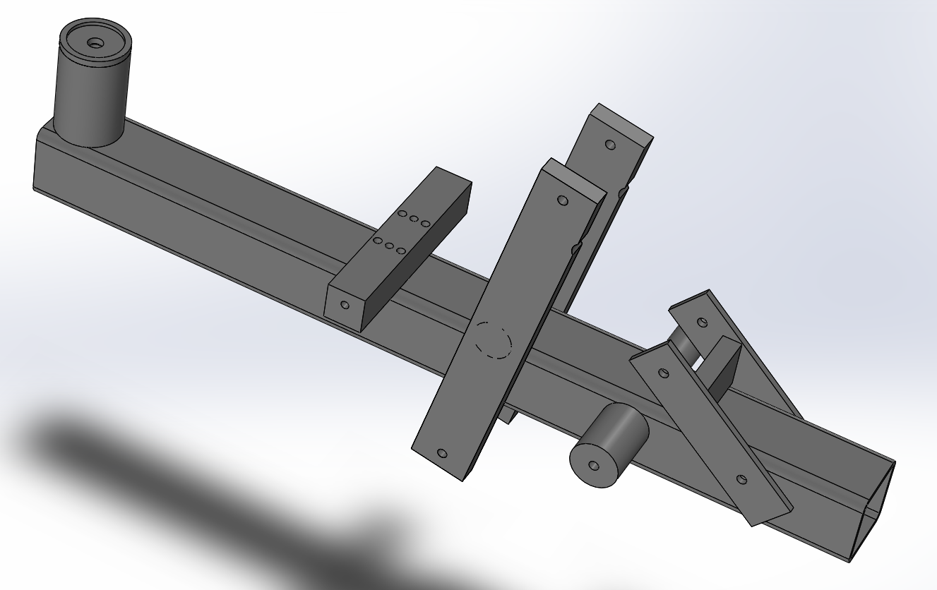
Although it’s not directly part of the bike, the first thing we did was to start the design of a support to mount the electric motor on a dynamo-meter (a sponsor allowed us to go to their facilities). As we will see later, the programming of the inverter is a fundamental task within an electric motorcycle, so we needed to be able to test the power given by the different changes we made to the inverter.
The dynamo-meter was ready to mount a vehicle on wheels, not with the motor directly with a chain for example, so we had to build something like a swingarm to be able to mount it.
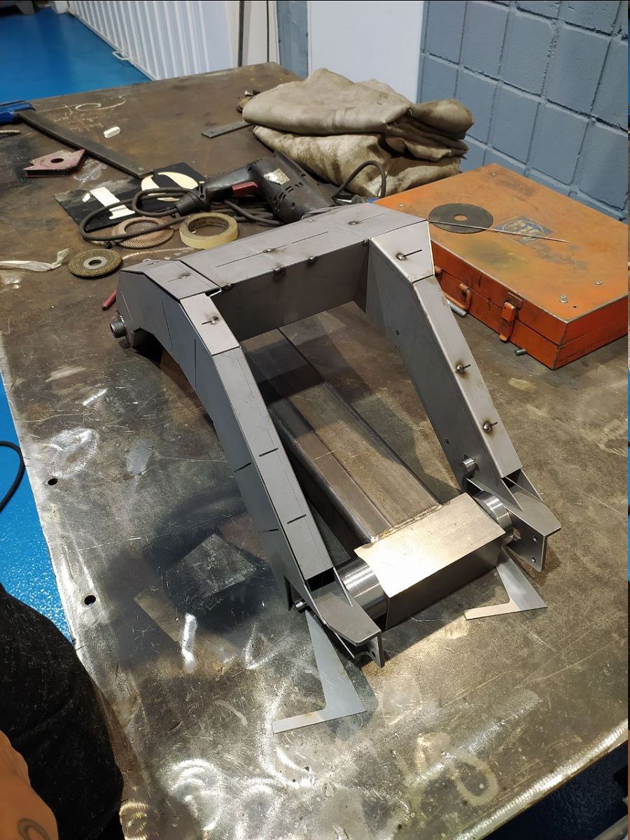
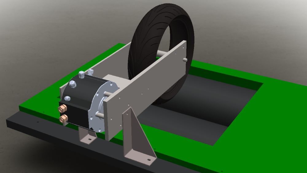 3D design of the dyno swingarm |
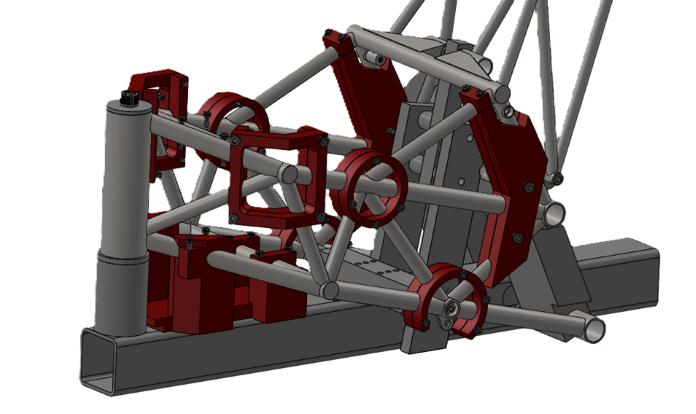
 Swingarm with all the elements on the dyno |
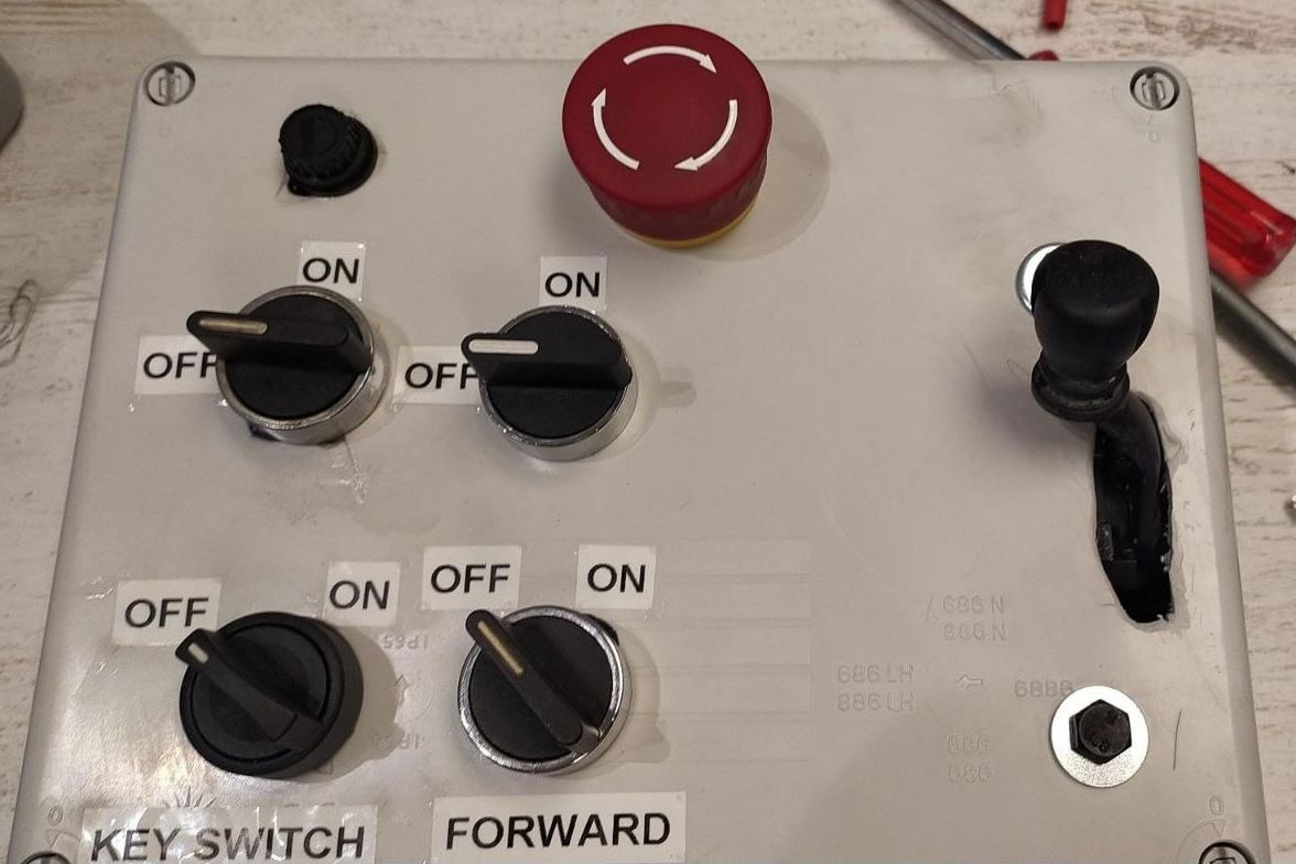 Control box for the inverter
To supply the inverter we used two lead-acid forklift batteries connected in series (96V nominal) as you can see at the back of the image, which allowed us to use the dyno for two or three hours continuously. With this we could start working on the inverter programming in parallel with the development of the motorcycle. The most important part of this step is that all the design will be conditioned by the work made on the dyno. Here we should be able to take as much power as possible from the motor with the lowest heat losses. Also we need to calculate the motor energy consumption to size the battery correctly. All this characteristics will be crucial to the correct design and decision making.
With this support manufactured, we could start with the design of the motorcycle while we worked on the dyno.
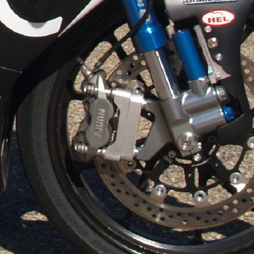
Front Brake and Forks
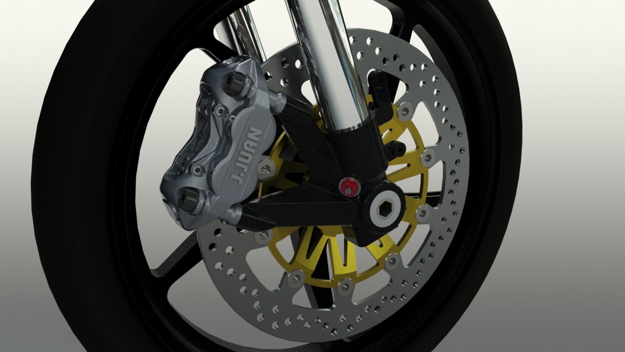
As mentioned previously, the organization gave us the front brake. We had a J.Juan front brake caliper of 4 pistons and radial mount.
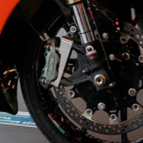
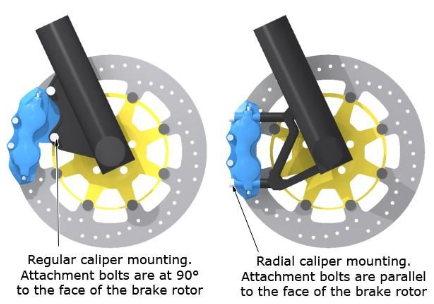 Radial vs axial caliper mount2
There are two types of brake caliper mounting, axial and radial. The caliper we have for this edition is radial and in the market there are mainly two (there are more) standard distances between the bolts of a radial caliper, 108mm and 100mm. We had a 100 mm brake caliper. Why does this distance affect to us? Due to this non-standard distance.
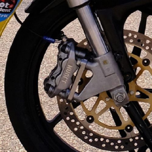
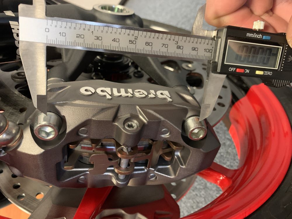 Example of 100mm radial brake caliper3
There are forks with different distances between bolts, so we have three options:
- Manufacture a custom mechanized part to adapt any fork to our caliper.
- Find a front fork with 100mm between bolts.
- Find a front fork with 108mm between bolts and manufacture an adapter.
- Find a axial mounting fork and manufacture an adapter for the caliper.
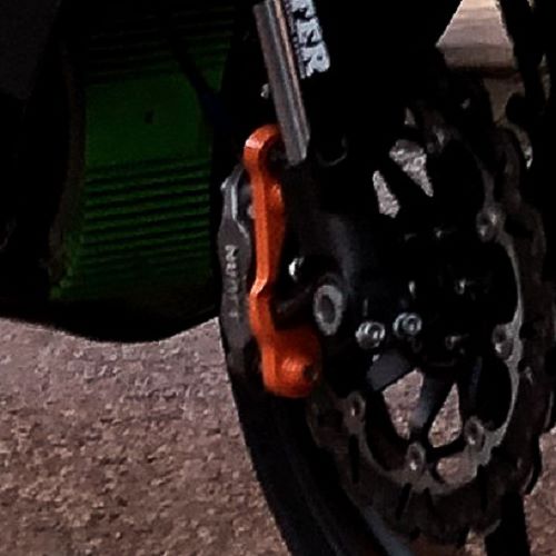
First option is expensive for us, so discarded. The third option was attempted by previous teams, with an axial brake holder:
 Example of 100mm radial brake caliper
This loses all the benefits of a radial caliper, so let’s try to skip this time.
Japanese forks are cheap and abundant in the market. There are high quality forks with cheap prices. The problem is that most of Japanese motorbikes have 108mm between holes. It’s a bit difficult to manufacture an adapter for this situation as there is no enough space for a clean anchor on the second screw (the one that is not aligned). Here there are some examples from other teams that adapted it:
 |
 |
 |
 |
This latest design by UPM is elegant but it’s built on an 84mm mount. These are usually racing forks and although they are the perfect option, this forks were very expensive for us.
The option of a 108mm fork could be a good solution. However, we were not completely convinced because the distance between the bolt holes is so small and 8mm is not enough offset between caliper hole and fork hole for the bolt.
On the other hand, European forks are perfect (BMW, KTM, Ducati, etc.) because they usually have brake calipers with a distance of 100mm between holes. The problem is that most of them are from big engine motorcycles, which makes it larger and heavier, and the fork is too long for our prototype.
After hours and hours of searching, we were able to find that the only two forks that could be suitable for our prototype were one from a Triumph Speed Triple 675 and another one from the Ducati 848 Evo.
With these forks we have a new problem. These motorcycles had 310mm and 320mm diameter discs and there were no discs on the market that met these specifications for our rims, for which only 296mm discs were available. This means that if we mount that fork and caliper, the brake disc will be small and the caliper won’t bite the disc correctly.
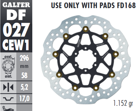 Biggest disc for our rims in the market4
After asking NG Brakes, we were able to get a custom build for our prototype with a 58mm inner diameter, 17.5mm rim cup and a 320mm disc. This means that we didn’t need to manufacture any kind of brake adapter. Also, with this design, we could mount the largest disc that fits on these rims (fixed by the organization as they give us the tires). We could say that we had achieved the most powerful braking system we could possibly create while also keeping design simple. This was reflected in the tests as we won the braking test over 45 teams.
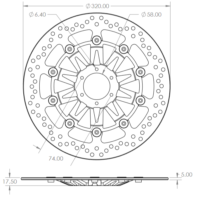 Front brake disc dimensions |
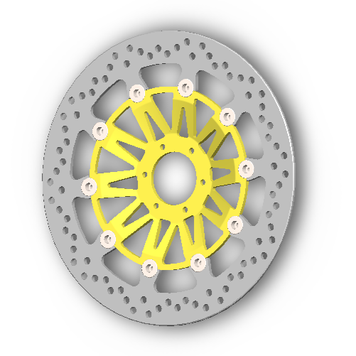 Front brake disc
|
With this brake disc ready, we selected forks from a Ducati 848 Evo. These Showa forks were ideal for the prototype though they were slightly longer than what we initially aimed for. However, they worked well.
Front Axis
With the brake disc, rims and forks chosen, we could start the front axis design. It should be noted that part of this design is restricted by the lower shape of the forks since they are commercial parts that we are not going to modify. It should also be noted that we were looking for a cheap and simple design. We didn’t need to quickly assemble or disassemble the front wheel at any time so the design was not focused on that feature.
For the design of the front axle, the order and restrictions applied to the 3D design were:
- Centering the front wheel axle with the front bar axle supports (concentric).
- Mounting the front disc on the wheel
- Mounting the brake on the right fork bar.
- Alignment of the brake pads with the brake disc.
- Symmetry of the left bar with the right bar with respect to the central plane of the wheel.
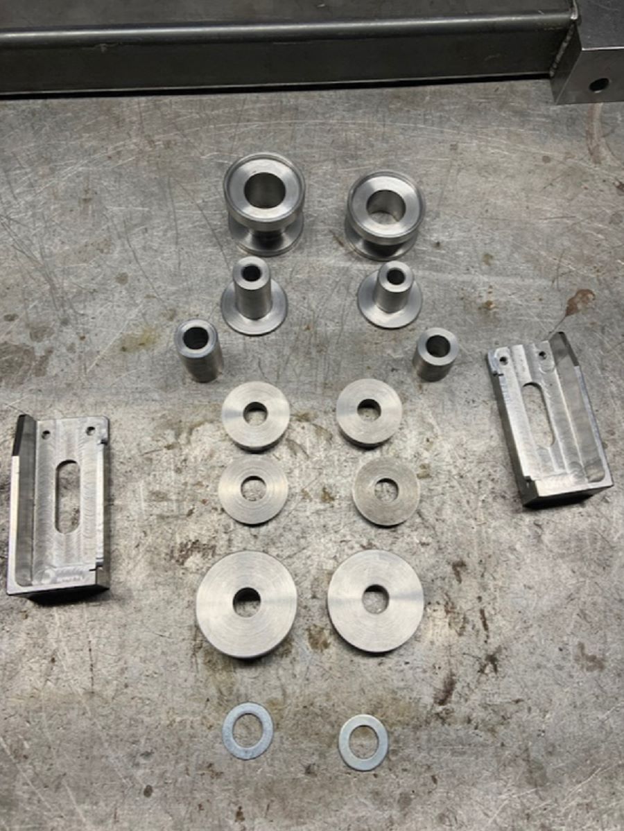
With this distribution we are ready to design the bushings and the axle.
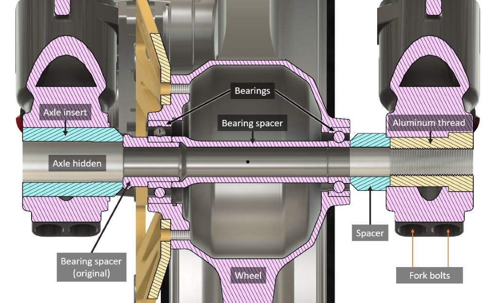 Front axis section view (hidden axle screw).
To begin, we need to examine the counterbore that exists on the right fork (shown in the image). This feature indicates that we can use this side as a tightening point for the assembly we are building with all the bushings.
The most technically correct design might have been to use a nut on the right side of the axle instead of tightening directly against the bushing (the yellow one). This would allow for a more secure tightening, but it would result in a less refined design, as the axle is limited to a 15mm diameter (due to the rim bearings).
It’s important to keep in mind that in this type of design, you should never tighten one fork leg against the other. The assembly should be compacted against one fork leg, with the other leg securing the axle in place based on its required position.
From right to left in the design, we start with a bushing (the yellow one on the right side), which will serve as the thread on which the entire assembly will be tightened. Due to the counterbore in the fork leg, this bushing will not be able to move to the left, effectively acting as a nut for the axle. Additionally, the fork legs will secure this bushing using two screws at the bottom, keeping it locked in place.
Next is the blue bushing, which works as a spacer between the rim and the fork. This distance is determined by the symmetry of the fork legs in relation to the wheel. The bushing is slightly inserted into the fork leg to center the assembly, making it easier to mount, and it also acts as a stop in the opposite direction, preventing movement to the right when the axle is tightened.
Afterward, we have the wheel bearing, an inner spacer, and the other bearing, followed by the final purple bushing, all of which are part of the original rim assembly.
Finally, we reach the blue bushing, which compensates for the difference in diameter between the fork and the axle. In this case, we used a 15mm diameter axle due to the wheel bearings. The original forks had a larger hollow axle, so we needed to supplement it. We adapted a factory axle from another motorcycle model by cutting it to the correct length and threading it to fit our prototype. That’s why the blue axle insert has its specific diameter—it matches the head of the axle we used.
When tightening it, the head of the axle will press against the left blue bushing (note the small counterbore), followed by the pink bushing, the next blue bushing, and the yellow one. This creates a compact assembly that is completely tightened against the right fork leg.
Finally, we tighten the left fork leg by securing it around the blue bushing, ensuring that the entire assembly remains in place. This process ensures the forks are perfectly parallel and properly aligned.
 Front axle assembly rendering
As for assembly, the tightening order would be:
- Lower screws on the right bar
- Axle insertion
- Lower screws on the left bar.
Note that if, on the other hand, we tightened the screws on the bars on both sides and then the wheel axle, the bars would tend to form a bundle between them and would not be completely parallel.
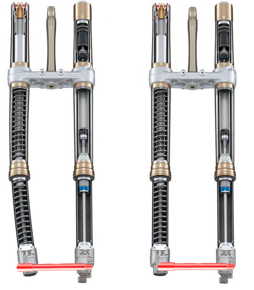 On the left of the image we can see the incorrect assembly of the front axle. This will cause the forks not to work parallel, causing malfunction and, in the future, a failure. On the other side, in the right assembly we can see how the axle is packed with the right bar and the left bar bites the axle in the natural position.
It’s also important the fact that we have modified the distance between the bars that were not from this bike. We will not be able to use commercial triple clamps, we will need to design and manufacture our own since the distance between the bars is completely different to the bike that had these bars. If we use standard triple clamps, the bar opposite the brake caliper would not be symmetrical about the center of the wheel, which would result in the prototype having the front wheel not aligned with the center of the steering axis. On the other hand, making our own triple clamps allows us to work on the geometry and make them with the offset we want.
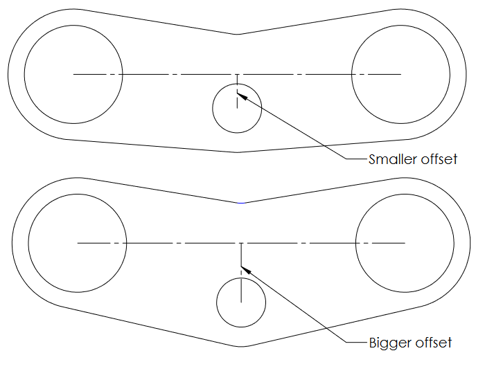 Playing with this offset give us different geometries and different prototype behavior.
This offset distance, as we will see later, will also influence the behavior and handling of the bike. With the front end sorted, it was time to start working on the geometry of the prototype.
Component Placement
Analyzing Previous Prototype
On previous edition, the bike geometry and components position was quite simple. The electric motor was in the same position as a petrol engine should be. Batteries are on the top of the motorbike, where the fuel tank should be. This is a lazy design has two main disadvantages:
1. The chain is too long
Normally, on a motorbike we have the current disposition:
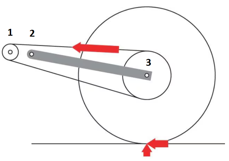
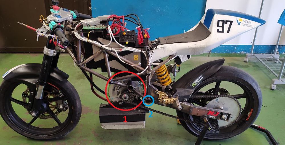
The engine output (1) is as close as possible to the swingarm pivot (2). This is because two main reasons:
- The chain should be as short as possible. It is a moving mass (an inertia) and that is not good for the behavior of the motorcycle.
- When the swingarm pivots, the distance between the point 1 and 3 (the chain length) changes. As close as we could keep the engine output to the swingarm pivot, we will minimize the length change.
 With this arrangement, the chain tension varies as the wheel pivots.
On petrol engine, this is not a problem because the diameter of the output shaft of the gearbox is small, so we can place the output (1) and the swingarm pivot (2) very close.
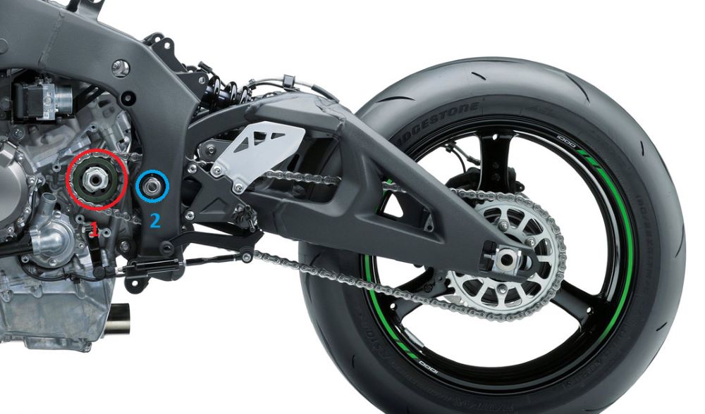
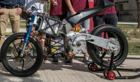
This is not possible with an electric motor. It has much higher diameter:
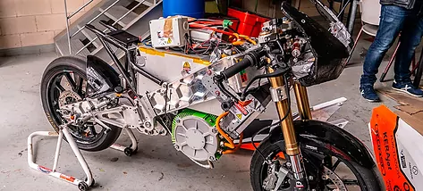
 Previous edition prototype
2. Battery weight is high
With the battery in that position, the center of gravity of the bike (COG) is very high. This means, when you lean in a corner, it’s more difficult to straighten the bike again, it tends to fall.
Looking for the Best Design
We had clear for the new prototype that there are two components that are important to fit in the correct place because of their weight and volume: the motor and the battery.
The battery is supposed to be bigger (we had a new motor, water cooled), so the volume and the mass was going to be bigger than the motor. Also, with the battery it’s possible to fit some spaces or give it the shape that we need. That’s impossible with the motor.
Analyzing Motor Position
We thought about two options for the motor keeping the shortest chain:
Make a chain forward
This means that the chain that transfers power to the wheel is not directly connected to the motor. There are one or more intermediate shafts.
For example, as Energica MotoE:
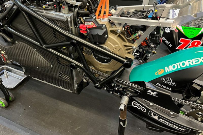 Energica MotoE transmission. It has intermediate gears to connect the chain output shaft to the motor.
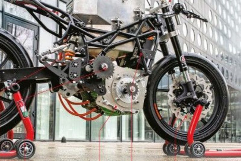 LEM Wroclaw prototype. There is a shaft between electric motor output and wheel.
The forward can be done by chain, belt or pinions. This gives three advantages:
- The output axis has smaller diameter, which helps to achieve shorter chain.
- Allows to pivot the motor to a lot of different positions such as upper to the axis output or in front.
- Allows to gear reduction. Normally these small electric motors work at high rpm (up to 8000), so if you have a direct transmission you need a big crown. With this gear reduction you can use a smaller crown.
Place the motor inside the swingarm
It doesn’t mean to fix the motor to the swingarm. We need to keep moving parts as light as possible. We were thinking about something like this:
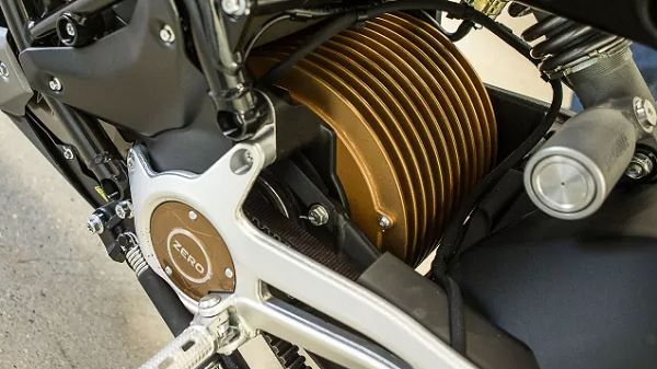 Zero motorcycles motor position |
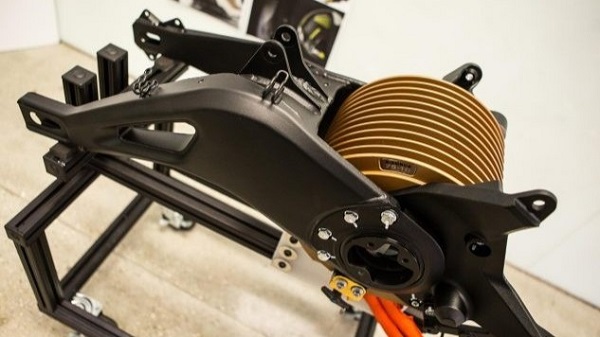 Zero motorcycles swingarm. Output shaft and swingarm pivot are aligned. |
As you can see, the motor output is in the same axis as the swingarm pivot. This is possible with an aluminium mechanized swingarm, but we wanted to make the swingarm with sheet metal as it’s cheaper and easier to manufacture it with our resources. This is also not the best option for anti-squat geometry as we will see ahead.
Analyzing Battery Position
The other important element is the battery. We wanted to keep it as simple as possible. This means, that if we can, we will build a cube to enclose it.
Due to lack of time, we needed some quick ideas for the design. After a lot of research we got some ideas from other teams. In general all prototypes converge on two designs:
Battery on top of the motor
 UMA Racing Team 2019-2021 3D model
 UJI prototype of 2019-2021 edition
 Kenji Racing Team prototype
This is probably the most traditional design, the one that had been used in the previous edition. It looks a lot like a petrol motorbike in which the tank (in this case the battery) is located above the motor. As you can see, there is a big cube on the top of the bike. It keeps the battery access very easy but we had to deal with a lot of empty space in front of the engine. This year the motor was water-cooled so we didn’t need to keep a direct air flow to it.
On the other hand, this design raised the center of gravity of the prototype a lot. The electrical calculations that we made gave us a larger battery than the previous edition so this design was probably not the most appropriate.
Battery in front of the motor
The other design was something similar to Zero motorcycles, keeping the motor between the swingarm and the battery. The problem with this design is that if a motorcycle were to be manufactured with a traditional layout, the prototype would be too long, which would worsen its agility in curves or low-speed maneuvers.
After analyzing prototypes from previous editions, I found a pattern or idea that could be developed. Introduce the motor into the swingarm to be able to make a shorter motorcycle. With this layout we do not lose the space that is limited by not being able to bring the swingarm pivot closer to the motor axis. Note that the design is not exactly equal to the Zero motorbikes. This one has the axis in front of the motor output shaft.
 2018 prototype of Guepardo Team from UMH
 2018 prototype of Guepardo Team from UMH
 UPM Motostudent EME-16E
We thought this design was better for keeping the COG low and chain length short, so we started working on it. Our idea was to use the motor as chassis as we have it there.
Geometry
Introduction
Maybe it sounds strange, but when you start drawing the prototype in the CAD software, a question arises, Where do I put the rider’s seat? And the footrests? What rake angle should I use for the fork? And what about the swingarm pivot point?
The book MotoGP Technology5, by Neil Spalding, explains the history of different MotoGP teams in the world championship since the arrival of 4-stroke engines. After reading the evolution of motorcycles from different brands such as Ducati, Honda, Yamaha or Suzuki, it is possible to understand the complexity of a motorcycle chassis. Neil Spalding perfectly explains the amount of testing that was carried out, bringing up to 3 chassis or different swingarms in a weekend to be tested and discarding some of them after just a few laps on the circuit.
Speaking about the chassis, the lateral flexing that the front end of the bike may have in a corner is not the same as the one that the rear end has. There are many parameters that vary the behavior, such as the wheelbase, the length of the chassis, the length of the swingarm, where the welds are made, flexing in different areas, the height and position of the rider, angles of the geometry such as the angle of the front fork, the position of the rear shock absorber and more. The problem is not only understanding all of this separately, the problem is understanding how each of these changes affects the behavior of the complete motorbike. To give us an idea of the complexity involved, racing bikes have different non-welded parts to be able to vary the geometry without having to manufacture a new chassis or swingarm. It has been proven that these joints negatively affect the dynamics of the bike, producing chattering (vibrations of the bike that appear at specific frequencies) between other problems. For this reason, some riders preferred to use the bikes with these welded and fixed elements. Reading all this characteristics made me feel that even the most advanced teams in the world with multi-million dollar budgets often did not know very well (or did not obtain the expected results) what they were doing. All this after many years of research. In some cases, even by trying radical ideas (changing geometries, heights, positions of the pilots etc.) they managed to achieve new lines of work that worked much better than those they had been working on.
My conclusion after all this was that the chassis was one of the parts of the prototype on which we had the least time to waste, since we were not going to have the resources, knowledge and time to be able to evaluate all these aspects of the prototype. In addition, everything I mentioned above pertains to MotoGP, bikes that reach speeds above 300 km/h and with close to 300 horsepower. Without being able to confirm whether it is my idea or not, probably all these parameters affect less a bike with less weight and power as would be the case with ours (it doesn’t mean that it doesn’t affect).
Basic Geometry
There are some basic measurements that must be established when designing a racing bike. These measurements directly affect the geometry and performance of the bike.
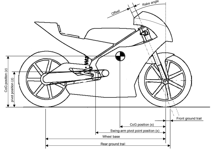 Basic geometry data
- Wheel base: Distance between the front and rear axles. A bike with a greater distance will be more stable on straights (high speed) but less agile in corners and slow zones. Having a greater distance will make the bike tend to wheelie less (with the little power that these bikes have, it doesn’t affect us too much) and the rear end will tend to lift less when braking.
- Rake angle: Angle between the vertical and the fork. Directly affects the trail.
- Offset: Displacement between the pivot point of the front axle and the axle of the same. A non-parallel offset could be made, although it is normal for them to be so. Racing bikes have non-welded elements that can be easily replaced to vary these measurements.
- Front ground trail: It’s the distance between the contact point of the wheel on the ground and the point where the line of the ground crosses the axis of rotation of the handlebar. This geometry is given by the angle and the offset. Generally, if we increase the rake angle we will make a more stable bike but lazier in corners. If, on the other hand, we decrease it, we will make a very agile bike but very nervous at the same time and not very stable at high speeds.
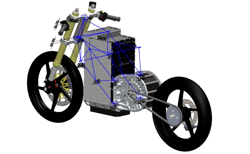
I remembered that a MotoGP engineer told me that they don’t leave the motorbikes with the steering straight when the motorbike is visible because other teams can get the geometry of the bike from one photo… perfect for us! We got a good amount of photos of some racing motorbikes from the side view. Of course there is some distortion because of perspective and camera lens but our result was convincing. Speaking about dimensions, this motorbike was supposed to be between Moto3 and Moto2 (as we saw later, it should be more like moto3), so here are the results:
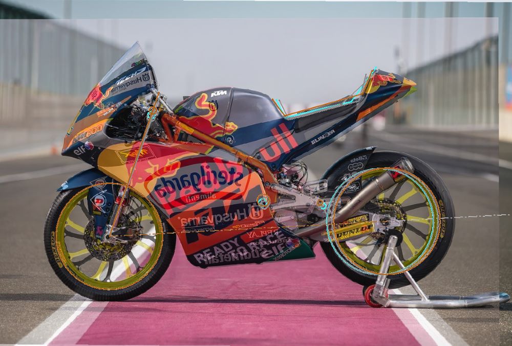 Different side-view photos aligned and extracted geometries
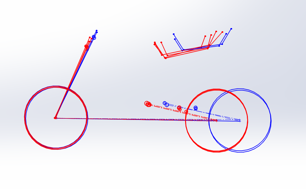 In red, Moto3 geometries, in blue, Moto2 geometries.
With this few examples we can say that we have something clear. Red sketches are from Moto3 bikes and blue are from Moto2 bikes. The conclusion we can draw is:
- As expected, Moto2 has longer wheelbase distance, making it more stable on high speeds.
- Moto3 bikes have a smaller rake angle and Moto2 a bigger one. With a smaller rake angle the motorbike should be more maneuverable but more unstable at high speeds. This makes some sense as Moto2 bikes are faster than Moto3.
- Forks are a bit longer in Moto2 and handlebar a bit higher too.
- The rider’s position in Moto2 is a little further back. This could be because the size of the engine, fuel tank, etc, not sure but it’s not the most important thing for us now. Also the footrests are further back, but it’s also the rider’s choice.
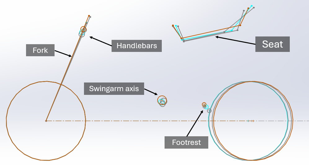 More Moto3 sketches
With this information, we have a clear starting point for geometry.
COG & Anti-squat
TO-DO
Clamps
As I mentioned earlier, due to the design of the front axle, it is not possible to use the original yokes of the bike to which the forks belonged to. Therefore it is necessary to design and manufacture custom ones for the prototype.
The only important measurement to focus on is the offset, that is, the distance between the suspension bars and the steering axis as we saw earlier.
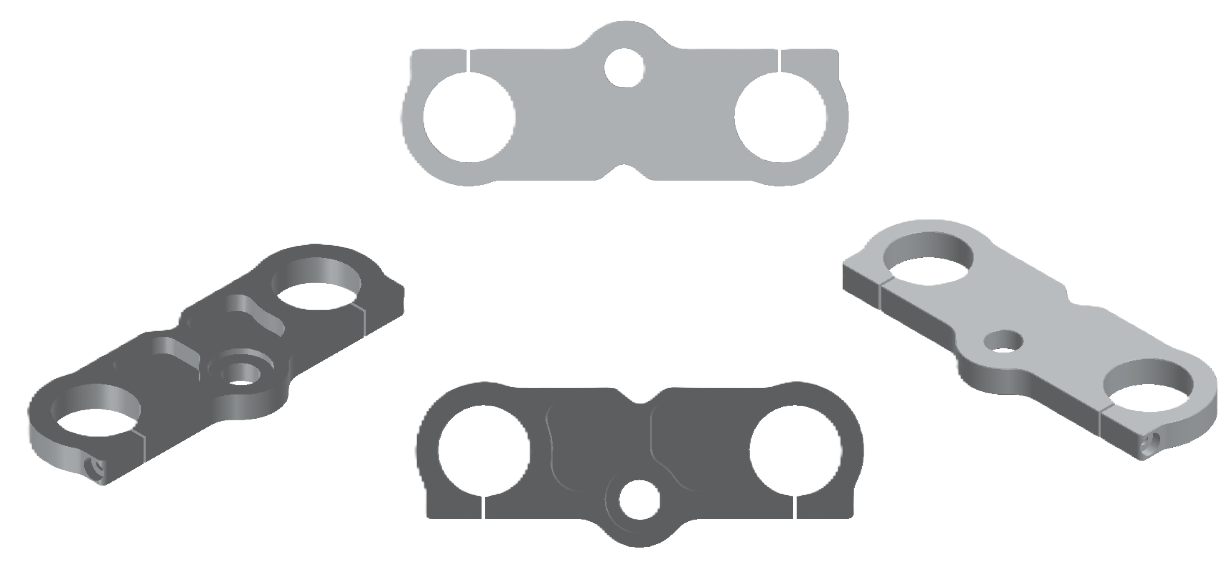 Upper clamps
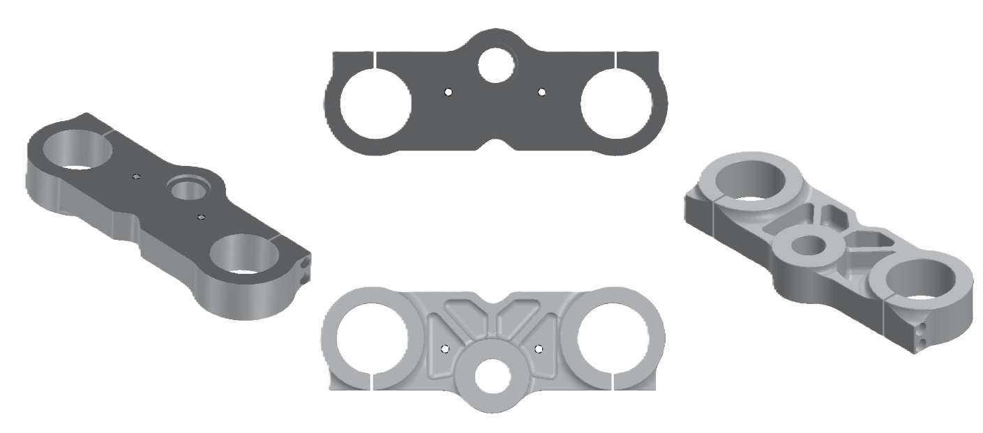 Lower clamps
Unfortunately we didn’t have time to work on optimizing these parts. I know that they are oversized and their weight could be reduced considerably.
Steering Axis
For the design of the steering axle we opted for a well-known and robust structure. The only possible disadvantage of this system is that it is not possible to modify the geometry once the prototype is assembled, but as we mentioned before, it is not something we are going to need so we opted to make it as simple as possible.
 Example of an adjustable steering assembly. As you can see in the image, there are some interchangeable pieces. With this parts, the geometry of the steering can be changed without big modifications on the chassis or the clamps.
Our design didn’t have this interchangeable parts, but the rest was similar.
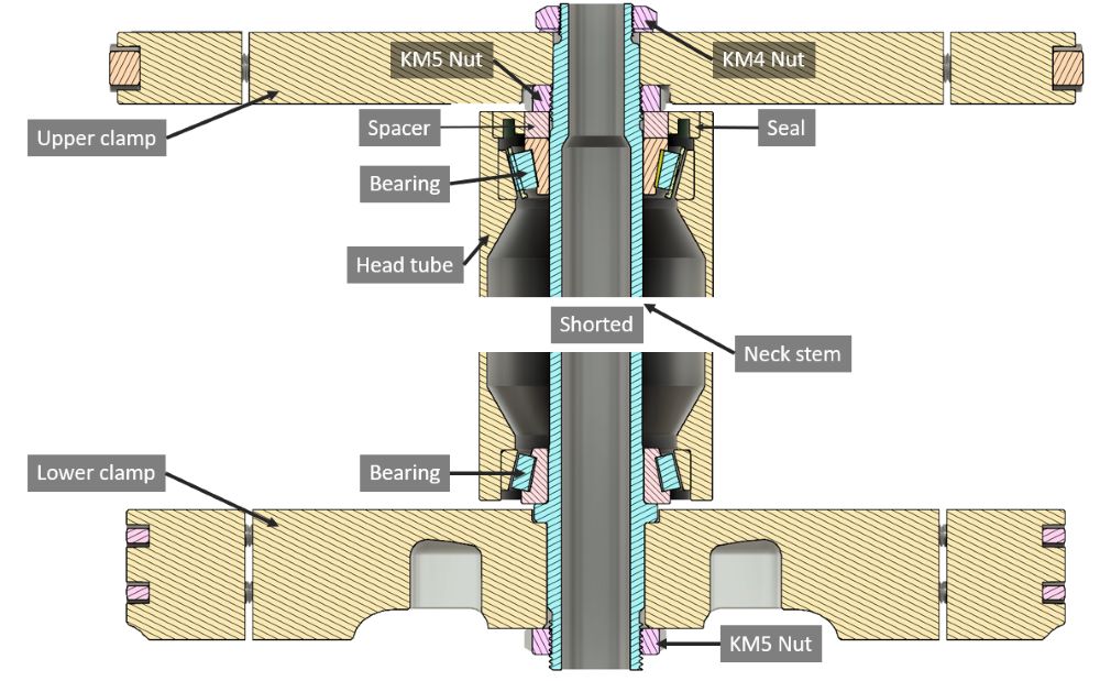 Section view of steering pipe
Starting from the bottom, we can see that we have a steel pipe in the middle (blue one). This pipe is tightened up to the lower clamp with a KM5 nut, so this two pieces are fixed between them.
Then we can find a conical bearing. The inner ring is fixed to the blue pipe and the outer ring is fixed to the steering pipe of the chassis. For this design, we used an inch SKF L44643 bearing on the bottom, with an inner diameter of 1 inch (25.4 mm). This means that the neck stem has a smaller diameter on the top so we can mount the lower bearing without problem.
On the top we have the other bearing, this time we have a SKF 30205 with an inner diameter of 25 mm. To cover this bearing we have a seal with a spacer inside to supply the difference of diameter and to allow a tolerance for the thread manufacturing.
All this is packed with a KM5 nut. This nut is important as it is the adjustment nut for the steering. We need to tighten it just right so that the conical bearings are not loose but at the same time not too hard.
Behind this is the upper yoke. This yoke is held in place with a KM4 nut and a small 1mm washer that acts as a spacer. Also this tightens the lower KM5 nut, preventing it from loosening.
With the steering axle design finished, we already have the front point of the chassis and all the geometries defined so we can start with the design of it.
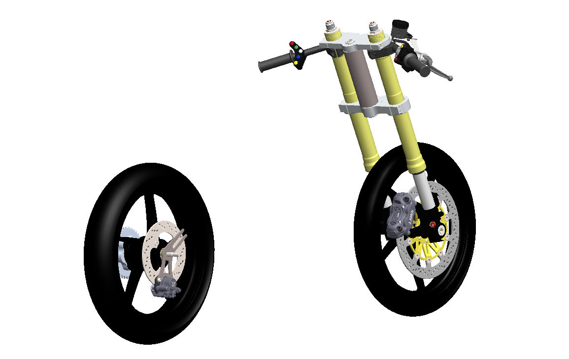 Finished front end
Chassis
I’m not going to extend too much this section. There are a lot of posts on the internet talking about chassis types, materials etc. For this prototype we could use 3 type of chassis:
- Beam (aluminum): It’s a good option but It’s expensive for our resources so we discard this one.
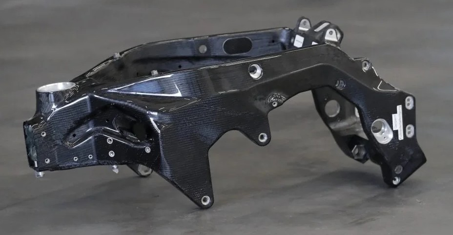
- Beam (carbon fiber): Another good option but It’s expensive, we don’t have the resources (machinery and companies that could help us with it) and also we don’t have the knowledge and experience. It’s probably the most complex one for design and manufacture.
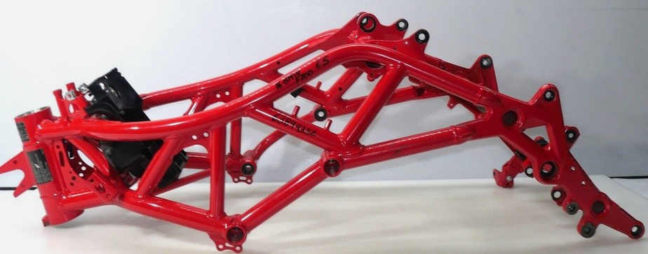
- Beam (steel): The team of a previous edition made one with sheet metal. In my opinion, it takes too much volume for this prototype, but it could be a cheap and easy option.
- Tubular (steel): It’s the perfect option for us. It’s cheap, easy to design, calculate and manufacture.
The material selected will be chrome molybdenum (42CrMo4). We will manufacture a tubular chassis with pipes of 16, 20 and 25mm of outer diameter and 1mm wall thickness. It is a cheap material, easy to weld and one of our sponsors had it in stock.
Design
The next step is to put the restrictions on the 3D CAD software. We have some mandatory restrictions such as maximum length, minimum distance between floor and fairing, etc. Also our restrictions, such as both wheels must be aligned on the same plane and tangent to the floor.
 Front view of restriction planes Front view of restriction planes |
 Restriction planes. Restriction planes. |
The next step is to place the electric motor. We still don’t know the position it will have in the prototype but we can start by aligning it with the central plane of the wheels. The order of proceeding would be, once we have the front wheel placed, we need to place the rear wheel aligned with the front. From here, the next restriction that applies to us is that the chain must be parallel to the central plane of the bike. Also, the end of the motor shaft (where the sprocket is placed) and the crown (rear wheel) must be aligned.
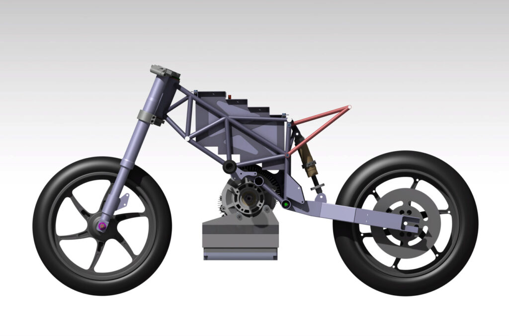
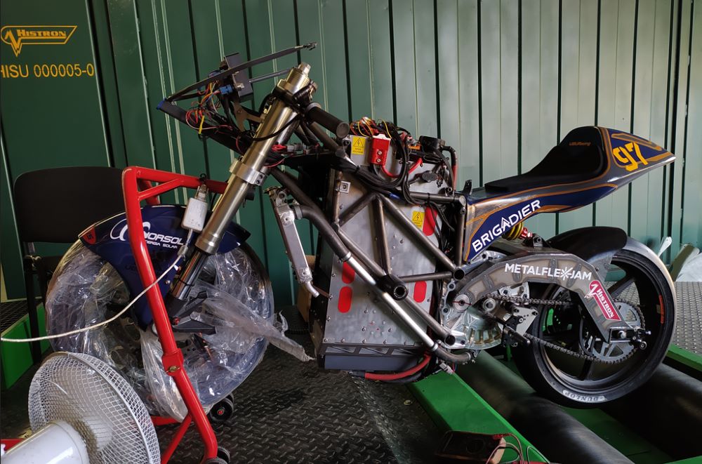
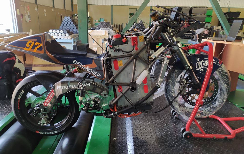
From this point we would have to start with the design of the battery since it is the part that will take up the most space and that will condition the rest of the design. During the process, that was the natural cycle although I will talk about the battery later. Let’s assume at this point that we have the exterior of the battery container designed.
As I mentioned before, we will try to use a layout in which the battery is vertical in the prototype and as low as possible, delaying the position of the motor as close to the rear wheel as possible. On the other hand, the idea is to take advantage of the rigidity that an element like the motor gives us to use it as a chassis.
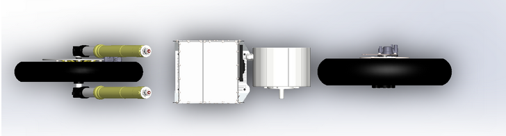
We don’t want to have more weight on one side than the other of the prototype. This means that the battery pack must be centered and aligned with the central plane of the wheels (and the motorbike). The next ideal situation would be to center the motor with the central plane of the bike.
 Battery and motor centered in the central plane of the motorcycle
In the swingarm section ahead, I discuss motor lateral placement and its limitations. This is the main reason why we will end up mounting the motor offset to one side as shown below.
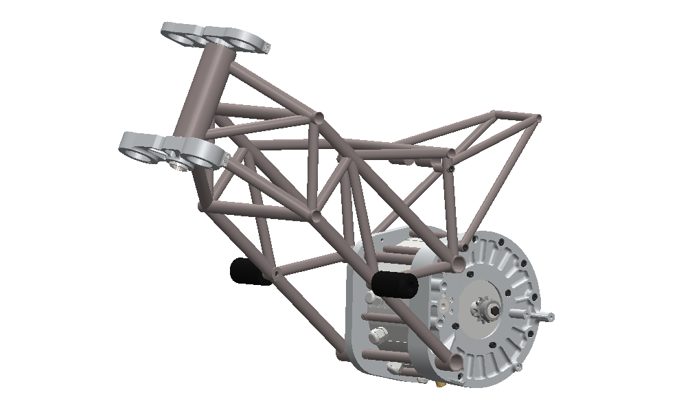
 Final component placement
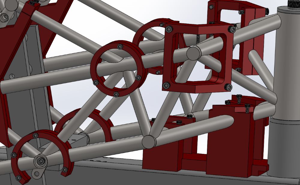
With the electric motor in place it was time to develop the idea of the chassis with the motor embedded. To do this, two side covers were designed that embraced the motor and to which the chassis and swingarm would be attached as previously mentioned.
 Initial design |
 Unfinished design |
 Final design. Note that the spacers between two sides are made with a pipe instead of a bar to reduce the final weight. They have a welded bushes on both sides with the threads.
Analyzing the design in more detail later, I realized that there is a lot of material left over in the rear area since the point of maximum load of these two pieces of aluminum is between the screws that connect to the chassis and the anchor points of the swingarm, but when you do not have previous experience in this type of design you always tend to secure and put more material.
With these motor covers designed, it was time to start with the chassis itself. To do this I started with a 3D sketch restricting the measurements we needed. One of the restrictions we tried to do was not to use bent tubes, both because of their loss of rigidity (straight tubes are better) and the complexity that would be involved in manufacturing them.
 Chassis sketch
After extruding the pipes and cutting them, we are left with the following design.
 Chassis design
It is well known that this is not the best way to technically design a chassis, but our time limit prevented us from working further on finite element analysis, structural optimization, etc. On the other hand, referring to what was mentioned above, we don’t have the knowledge or the resources to analyze a chassis behavior and how it works in a real environment so I didn’t want to waste too much time on it. Also, the problem is not to give more or less lateral deflection, or stiffness in X points. The problem is how can we know how much deflection you want to have. We don’t have the capacity and knowledge to get and analyze that data.
Some Chassis Design Details
Here you can view a sectional view of the unions between the chassis and the aluminum-machined parts covering the electric motor.
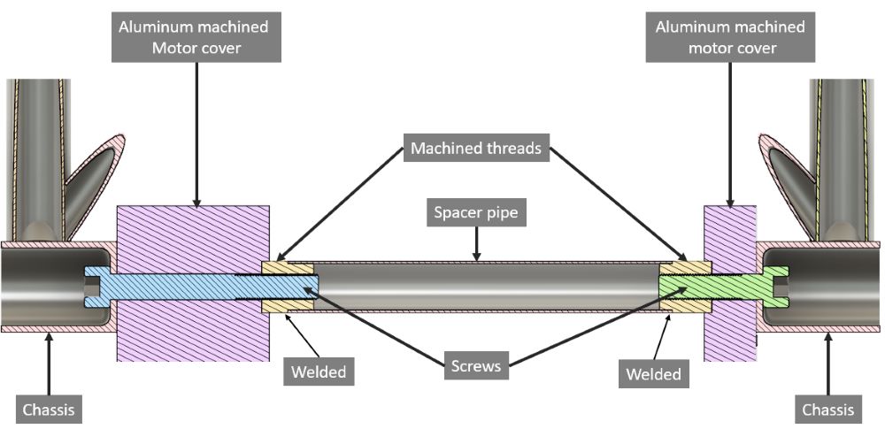 Detailed view of the join between chassis and motor cases
For the union between the machined aluminum parts, we manufactured 2 bushings with an internal thread. This parts were welded to a 16 mm diameter tube with 1 mm wall, making the design lighter than with a big screw for example.
Chassis Jig
Once the chassis was designed, it was time to design the welding jig. This is a structure to keep the position of the important points of the chassis during welding. This is because welding reaches high temperatures that cause the steel to twist and move from the original position. With the chassis jig we ensure that these points do not move during welding process.
 Previous edition jig
We had a jig from previous editions so we tried to reuse it by manufacturing some new parts and machining different sections.
 Chassis and colt final design
A new feature implemented for the manufacture of the chassis was the use of 3D printed supports to hold the pipes during welding. The purpose of these supports was not to have great resistance. We wanted simply to hold the pipes in their position during the initial phases of welding pointing, as well as to avoid having to hold them by hand and to be able to preview the reshaping before welding.
 3D printed supports for chassis manufacturing
 Pre-assembly of the chassis. 3D printed supports in order to position the pipes before welding the chassis.
Swingarm
The swingarm was designed at the same time as the chassis since one influences the other in certain decisions such as the position of the rear shock absorber or the swingarm axis.
Introduction
As I mentioned before, the initial idea was to manufacture the swing arm with folded sheet metal. This has many advantages, although the only drawback I see is space. It is a hollow structure with low weight but has a larger volume.
The first thing was to define the geometry it would have. After several options, we decided to make a banana-type swingarm.
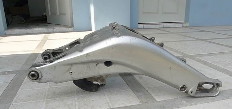 Example of banana swingarm
With this type of swingarm we would have sufficient length and rigidity, since the other option was to make a traditional swingarm but we would not have space to place the shock absorber apart from being a very short swingarm. In addition, this design would allow us to bring the wheel closer to the electric motor, allowing us to shorten the wheelbase of the bike as much as possible.
To do this, I searched for information about the rear wheel travel that motorcycles usually have. It was around 130 mm6.
The first thing was to select a shock absorber to know its data such as extended length, compressed length and travel. For price and features we bought a second-hand MUPO GT2.
Rear Shock
TO-DO: Rear shock geometry and spring calculations.
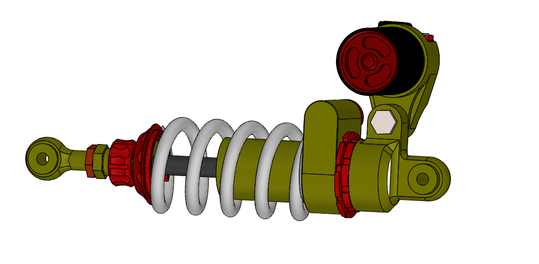 3D model of MUPO GT2
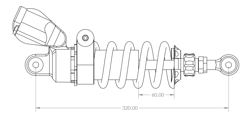 Total length and travel distance
With this shock absorber we had a travel distance of 60 mm. This would be one of the restrictions to be applied to the design. The other restriction would be the maximum travel of the rear wheel that was around 130 mm. Of course, there is nothing scientific about this “assumption” but we have to remember that there wasn’t too much time remaining to finish the project.
Swingarm Geometry
For this purpose, we prepared a sketch with the maximum and minimum positions that the geometry would have to comply with:
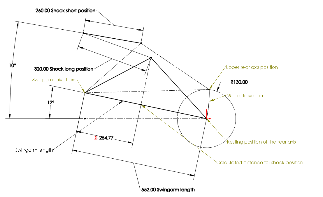 Swingarm geometry
Some defined values are the 12º between the ground parallel and the tilt of the swingarm. This is given by the geometry obtained from the photographs. The 10º between the ground and the shock absorber in the most retracted position is to restrict the sketch in a position that was valid for our design. The distance between the output motor shaft and the swingarm pivot axis (97 mm) is calculated by the largest sprocket we expected to mount (14 teeth) and trying to keep both points as close as possible.
Finally, the position in which we must place the shock absorber on the swingarm is given by the length that the shock absorber travels in the compression process (60mm) and the length that the rear wheel should travel during that journey (130 mm). With this calculation we get the distance of 254.77 mm.
Chain Geometry
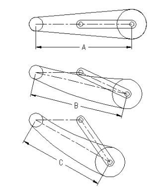
The next step is to calculate the position of the motor sprocket for chain elongation. Due to lack of time we could not accurately calculate the anti-squat so we took the decision to align the motor sprocket with the center position of the swingarm. As mentioned above, the idea is to mount the electric motor as near to the rear wheel as possible. This means that we will have an inverted situation respect to the electric motor pinion and swingarm. By having the sprocket inverted respect to the pivot point of the swingarm, this system works the opposite of the above mentioned, i.e. when the 3 points are aligned we have a shorter chain and when the motor sprocket is misaligned we have longer distances.
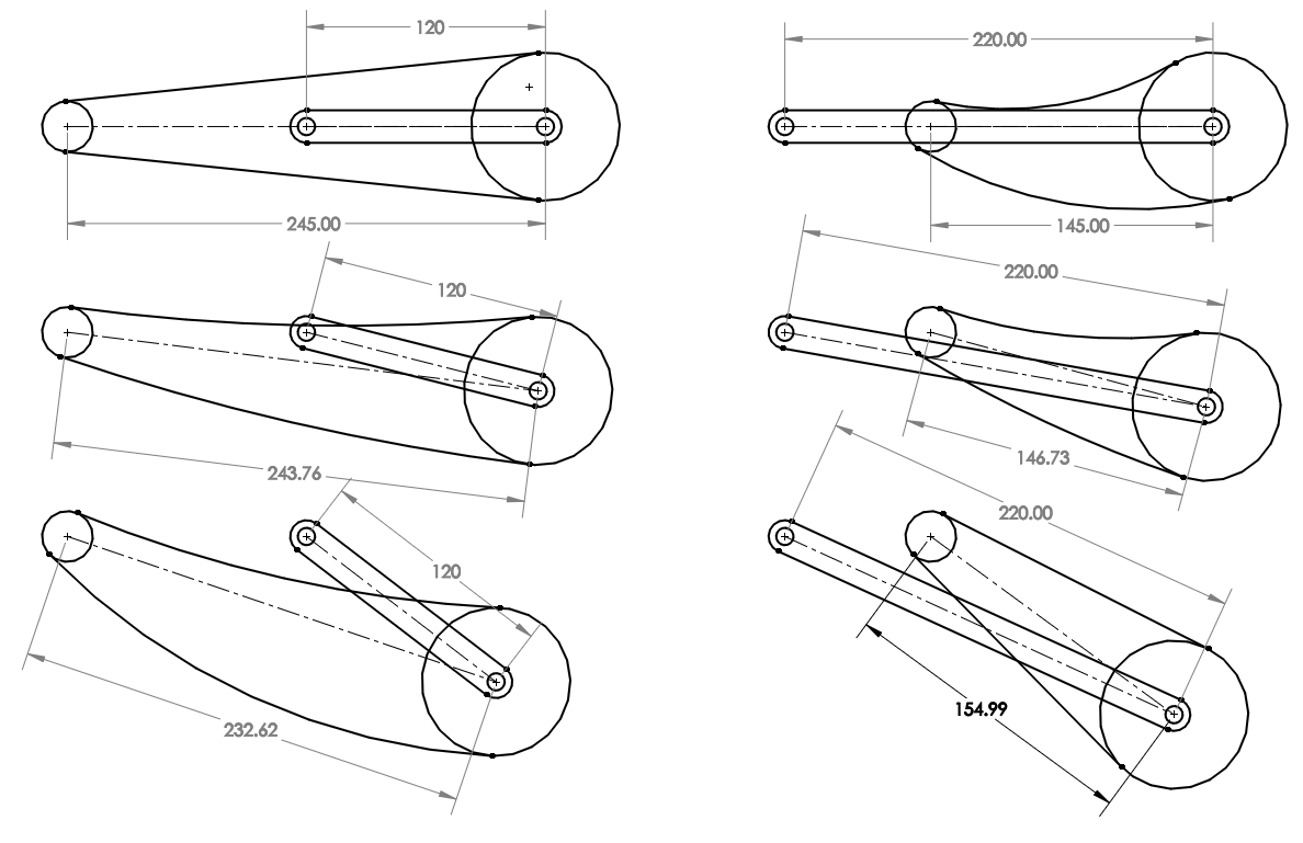 Common swingarm vs inverted swingarm. Note that on the normal one when the pinion, pivot point and rear axis get misaligned, the distance between the pinion and the rear axis is shorted meanwhile on the inverted swingarm it has the reverse effect.
We decided to align the sprocket with the swingarm pivot point and the rear wheel when the suspension is on the 25% of the complete travel (SAG). This will allow us to have the chain with the maximum tension on that point.
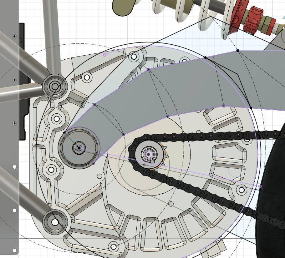 The soft blue area reveals the position of the swingarm on the most compressed position.
As you can see, the electric motor pinion is a bit up from the line between the swingarm pivot and rear wheel axis. This is the rest position without load.
Swingarm Design
With this data we already had the main points to start with the design: pivot point, rear wheel axle and rear shock absorber point. The first thing was to start designing it as a solid part. From the side view it was quite simple, taking care that we were going to manufacture it in folded sheet metal.
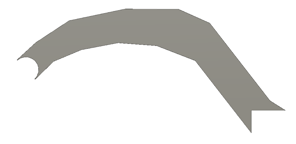 Lateral shape of the swingarm
The biggest challenge was on the top plane. It would not be a symmetrical swingarm because the anchor points to the chassis were not aligned with the anchor points of the rear wheel. Keep in mind that it’s important to keep the rear axle width as short as possible. For achieving it, we couldn’t design a straight swingarm on both sides.
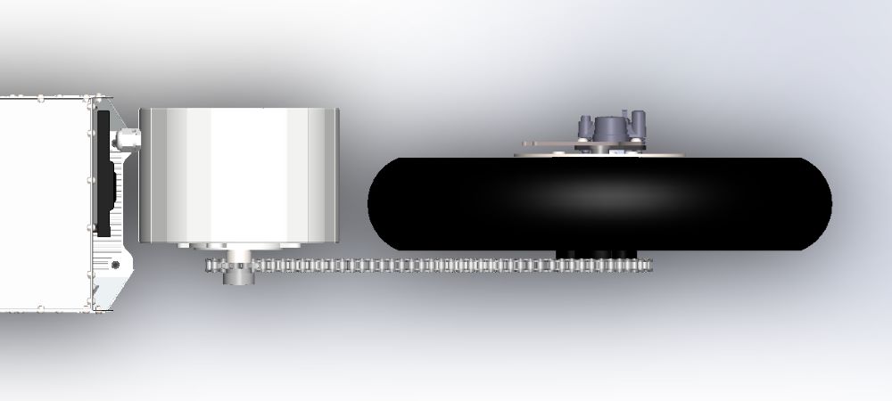
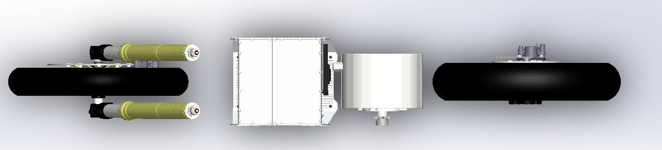 Electric motor and battery centered with the middle plane of the prototype.
We can start centering the motor with the wheels. The main issue of this design is that the chain would be too far from the rear wheel.
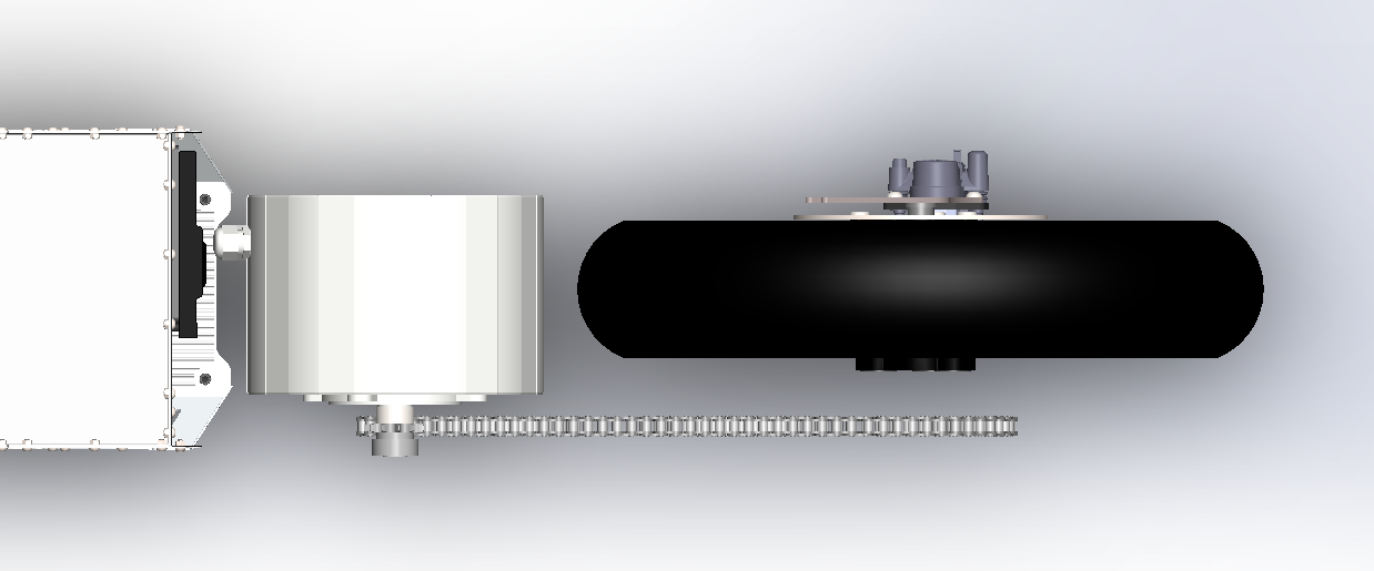 Electric motor aligned with center plane of the motorbike. Note the space between the chain and the rear wheel.
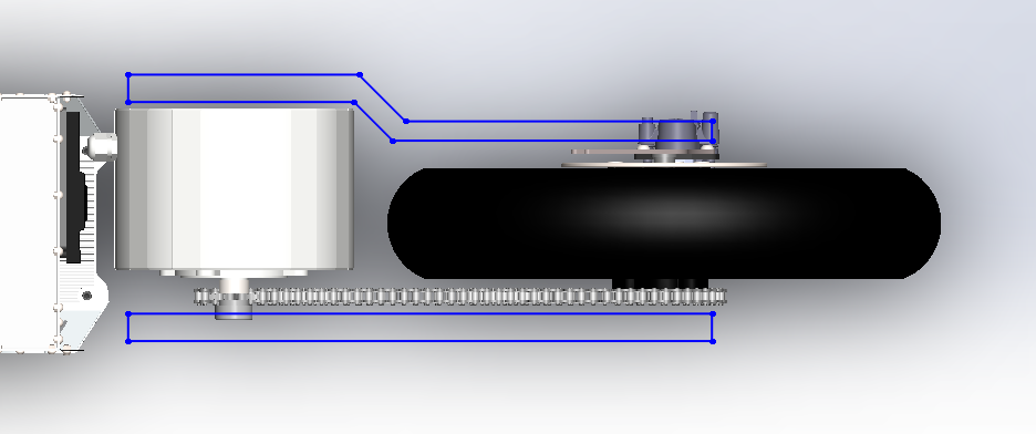
 Sketch of the approximate position of the swingarm with this arrangement.
On this position, the distance between the rim and the chain is too high. In addition, the left swingarm would be exposed to the outside as well as the rear axle while the right side would have plenty of margin.
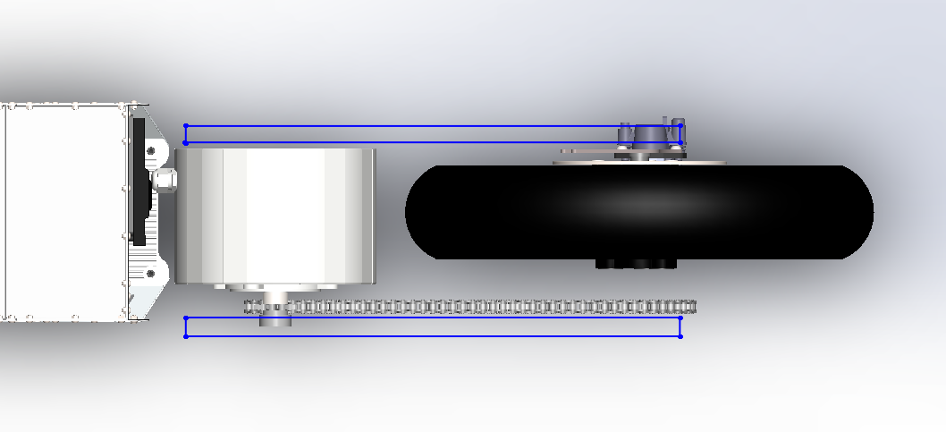
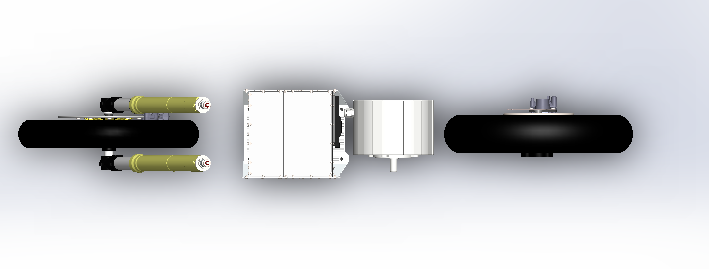
The opposite option would be to align the electric motor on the position where the chain should be.
 Chain aligned with the original rim sprocket.
This configuration is perfect for the chain. The problem is that the electric motor is displaced to one side, unbalancing the weight to one side of the motorbike. In addition, the swingarm would be very exposed in the front area on one side.
 Sketch of the swingarm in this arrangement.
Also we need to be careful with this designs because there will be an extra thickness of the aluminum cover parts of the electric motor. This will increase the issues of this designs making the swingarm more outside than expected.
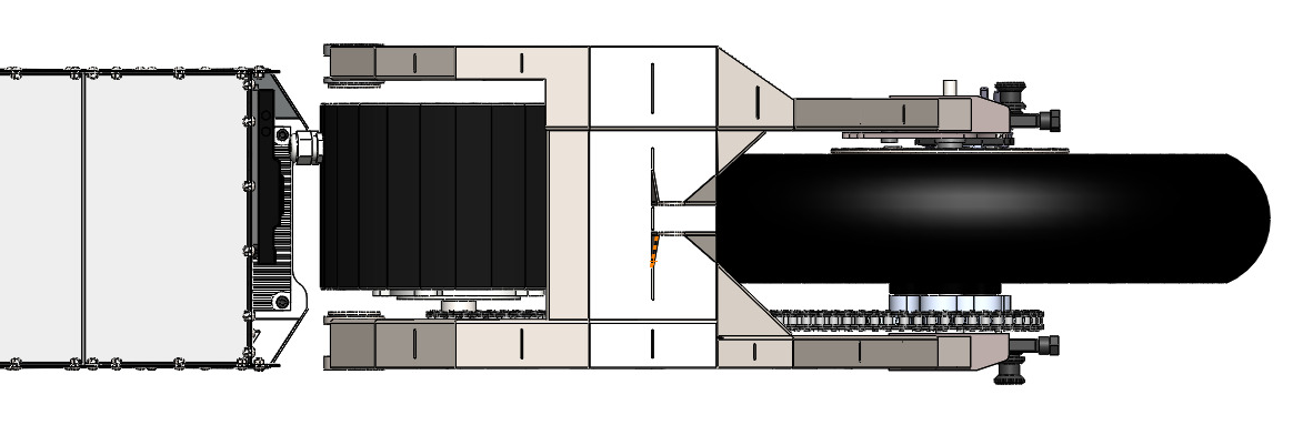
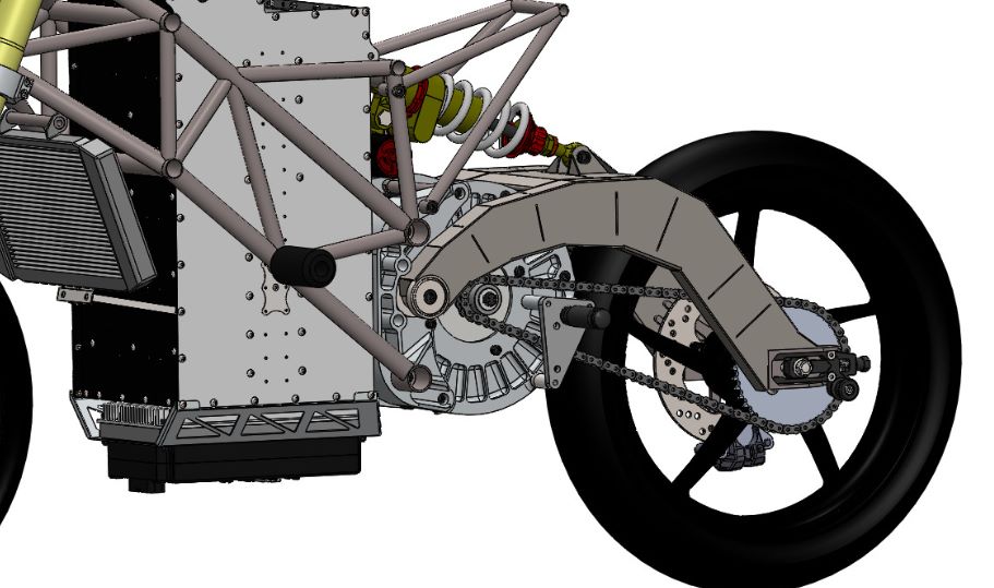
The solution is to find a middle point between two designs. A point where the motor is enough centered to allow us to put the swingarm front arms on both sides without protruding too much, but at the same time with the crown not too spaced from the rim.
 Final placement
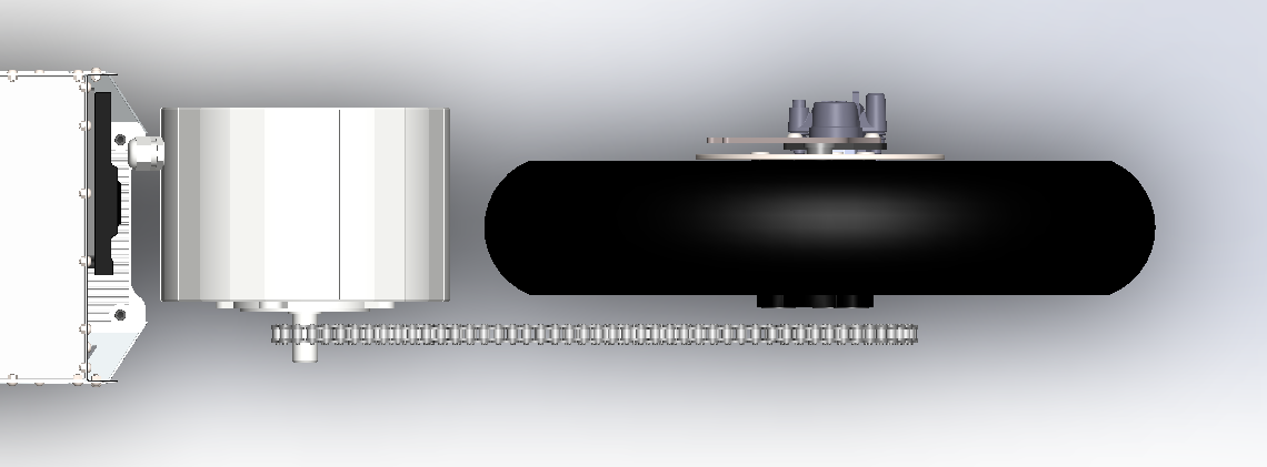 Final chain position
 Swingarm on final position
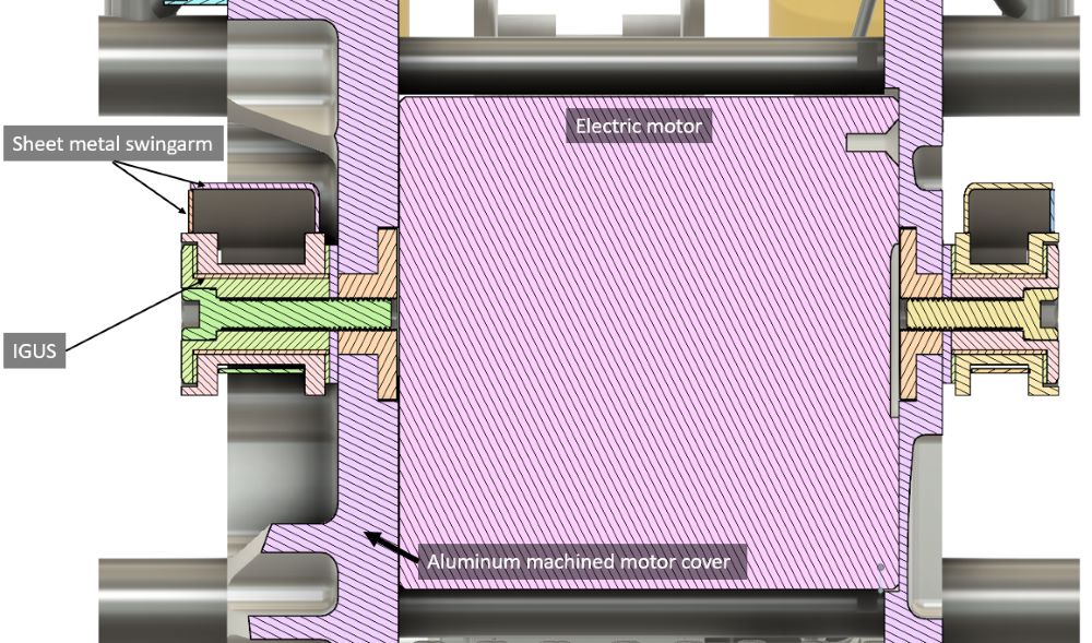
After analyzing different alternatives for the swingarm axle, we decided to use IGUS bushings. These are anti-friction plastic bushings. It’s much simpler system and lighter than using bearings. That’s enough as this prototype is not going to be used too much or on bumpy roads.
After working on the initial idea, we ended up with the following design:
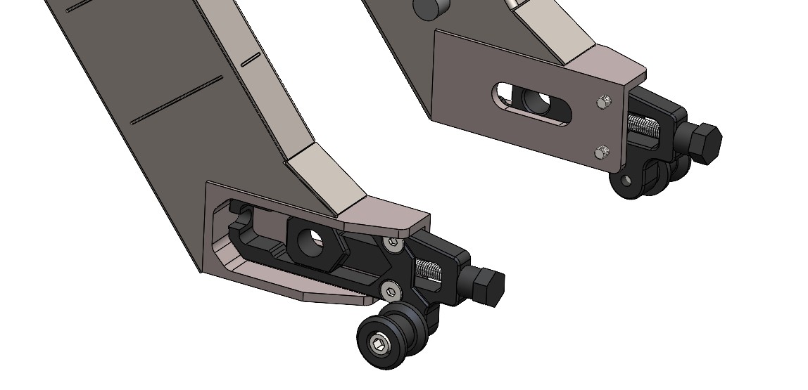
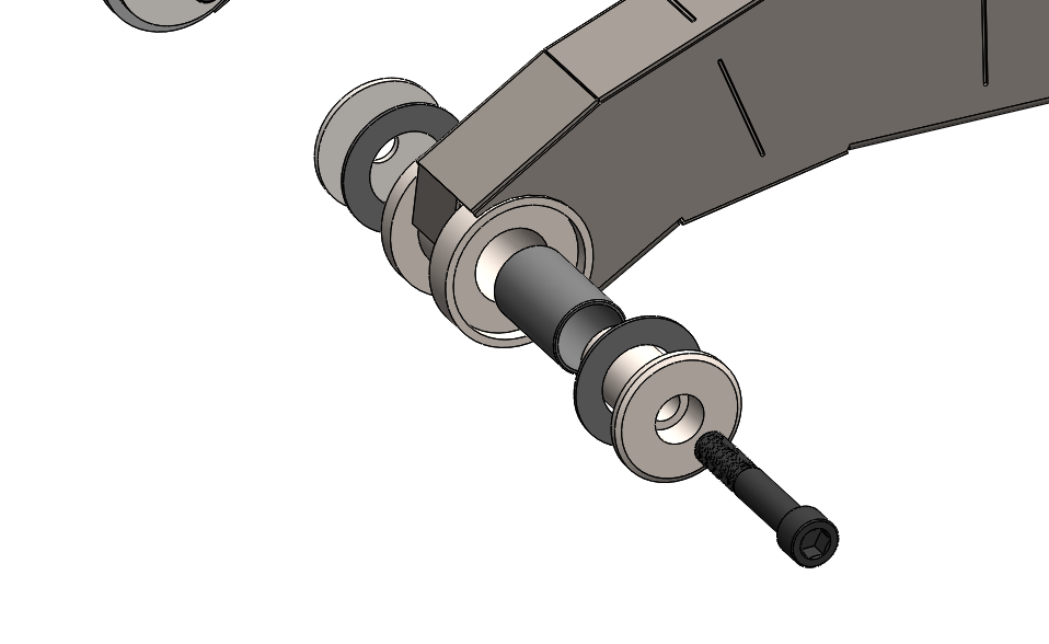 Exploded view of the swingarm pivot
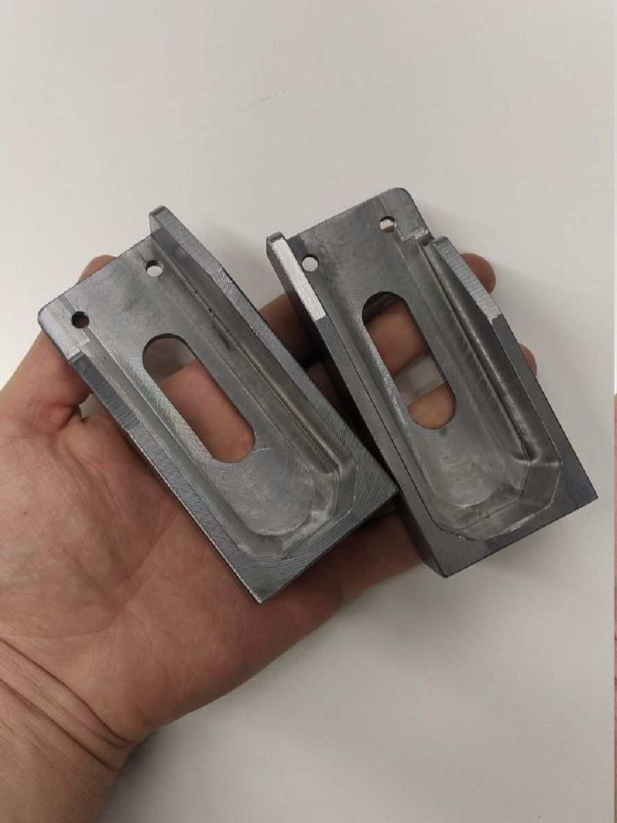
The challenge was there would be no swingarm axle between two sides. We needed to design two aligned anchors to hold the swingarm and pivot on them. The motor covers were going to be manufactured of aluminum and it was not the most suitable material to withstand the forces to which these threads would be subjected, and less on a thread that also had to be fine pitch due to the little space we had to not make this part too wide.
To achieve this, we designed two steel auxiliary parts that would be bolted to the aluminum machined motor cover with a M12x150 (fine pitch) thread. With this, we distribute the load over the machined aluminum parts and ensure a solid thread for the axle.
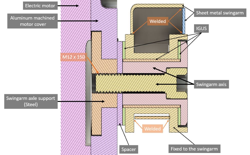 Section analysis of the swingarm pivot.
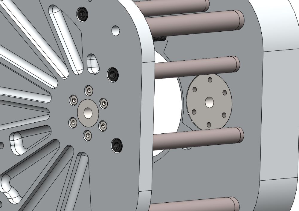 View of the steel inserts on the aluminum electric motor covers.
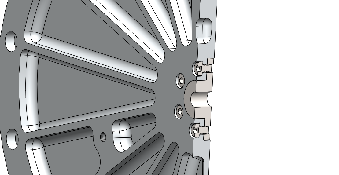 Section view of the steel inserts.
 Section analysis of the swingarm pivot axis.
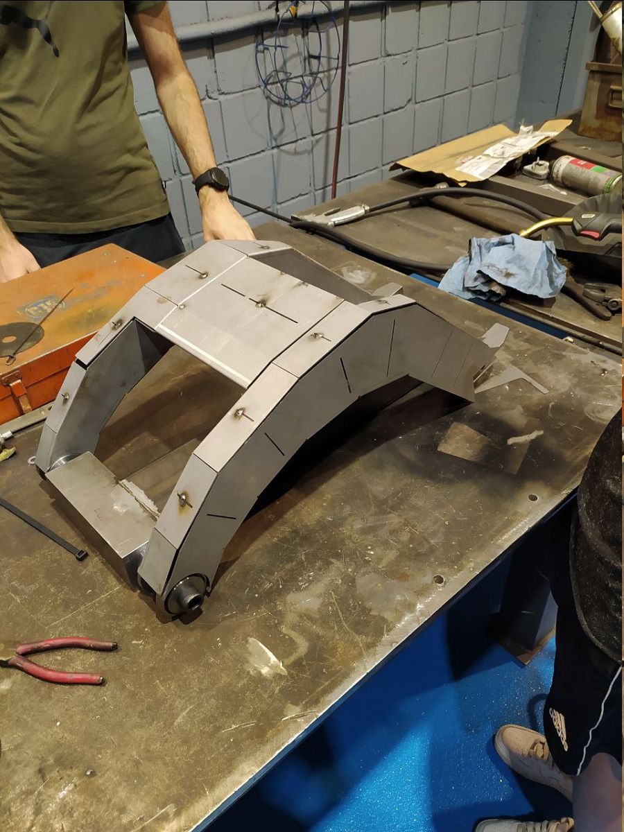
With the solid design finished, it was time to convert the swingarm into sheet metal. For doing this we tried different software such as Fusion360 and Solidworks. Solidworks worked better for us and after many attempts, this was the final result:
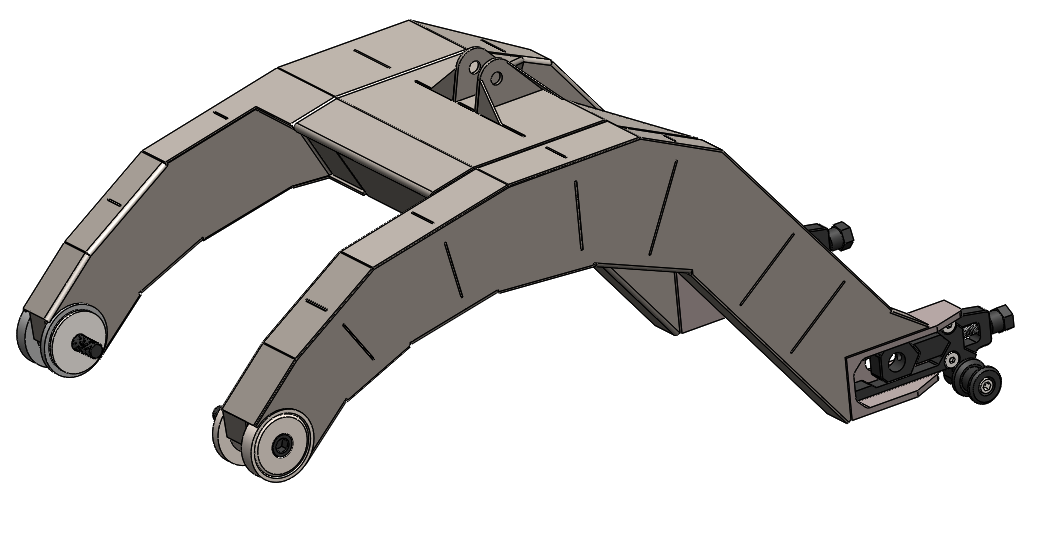 Swingarm render
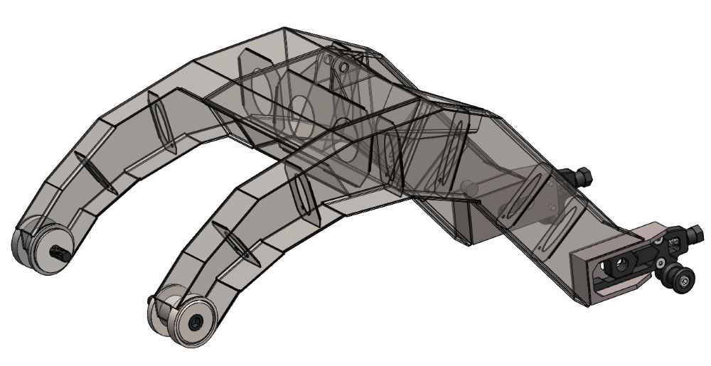 Transparent swingarm render
 Transparent swingarm render
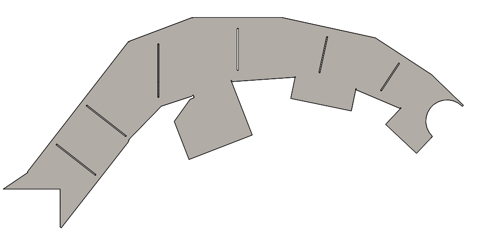 Unfolded swingarm side. This is resulting part from laser cutting.
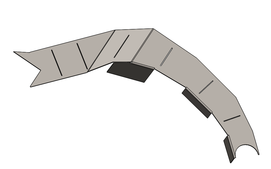 Folded swingarm side
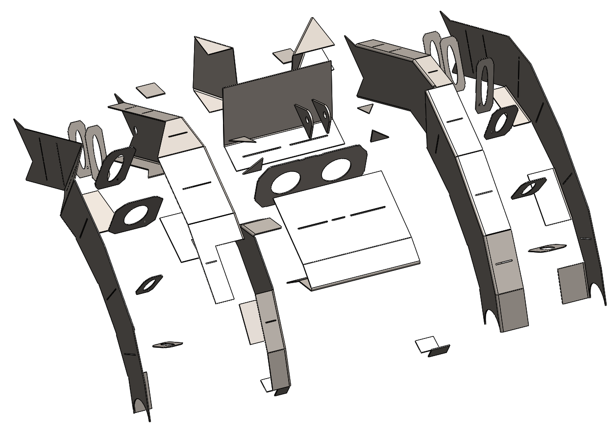 Swingarm exploded view
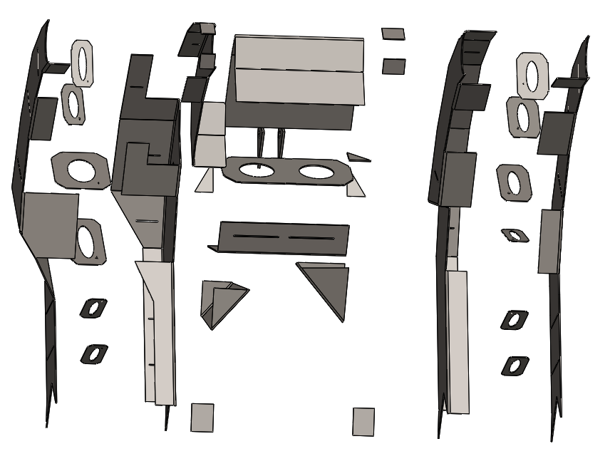 Swingarm exploded view
To secure the rear axle, two machined parts were designed and welded to the swingarm. On the other hand, aluminum chain adjusters were purchased to adjust the chain tension.
 Rear axle tensioners
Rear Axle
With the swingarm design completed, it was time for the rear axle.
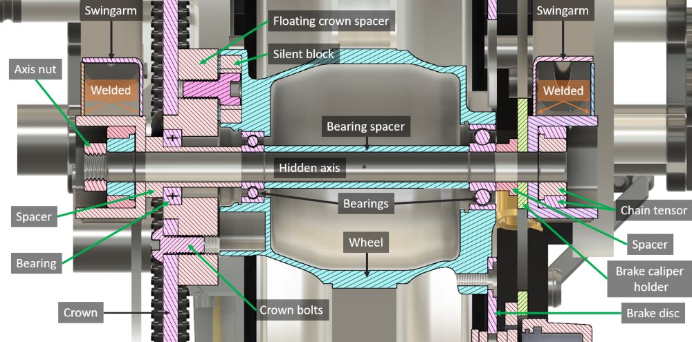 Section view of the rear axis
Starting from the right to the left of the image, we have to note that we have 4 fixed elements that are already defined:
- The left swingarm support.
- The right swingarm support.
- The rim with its bearings.
- The position of the chain.
These 4 elements are given by the previous decisions made in the design. Therefore, we will apply the same strategy as in the front axle, to go supplementing the spaces based on the measures that we have. To do this, starting from the right to the left:
We have the swingarm support together with the chain tensioner. Next we can find the support for the rear brake caliper which acts as a spacer. Keep in mind that the thickness of this piece is given by the position of the disc and the brake caliper. In this case it was a standard thickness of 5 mm so we were able to manufacture a laser cut piece.
Next we find a spacer that supplements the distance between the brake support and the wheel bearing. Along with it’s the inner spacer for the rim bearing and the other bearing. This parts are from the original rim. Up to this point it’s a normal design, very similar to the original one for this wheel. The difference becomes in the chain support. This rim is designed to work with the chain close to it, but due to the restrictions explained above, we cannot bring the chain closer to the rim, so the sprocket remains separated.
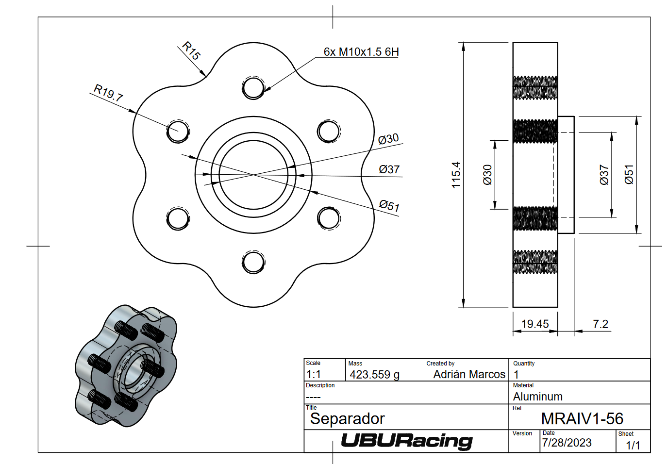
To solve this issue, I designed an aluminum spacer:
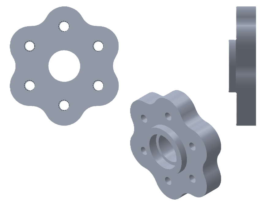 Crown spacer
This spacer has a bearing aligned with the chain to carry out the load on it. The original design of the rim had 3 silent blocks for drag the rim from the chain. As we didn’t have too much space on the outside of this spacer, I designed the spacer with 6 holes. 3 holes to fix the crown to the spacer with screws and other 3 holes to drag the rim from the spacer. This also keeps it floating with the silent blocks.
Transmission
As mentioned above, there are different alternatives for the design of the transmission for a motorbike. The following are some of them with their advantages and disadvantages:
Direct chain drive: This option is the simplest. It consists of connecting the chain directly between the electric motor and the rear wheel. It has several disadvantages compared to other systems, but the main advantage compensates them. Following the rule KISS (Keep It Simple, Stupid), the main advantage is their simplicity. We should keep in mind that the goal is to build a prototype. It’s a complex vehicle that is designed in a short period of time and we don’t have time to change this systems, we need something working on the first attempt. It’s the main reason why we selected this system.
Transmission with chain/belt/sprocket: This option consists of having intermediate sprockets between the electric motor and the wheel. This has disadvantages such as taking up more space and the loss in performance that this intermediate mechanisms may have. On the other hand, it has two great advantages: the electric motor can be positioned in a different place than usual and the components can be distributed more freely inside the prototype. Also, the size of the crown can be reduced making intermediate reductions. Note that these small electric motors run at high revolutions (usually up to 8000) which makes it necessary to place a large crown on the wheel.
 Example of direct transmission with big crown from US Racing.
Gearbox: This option offers the most advantages, but on the other hand it’s the most expensive and complex system. It’s well known that electric motors offer a lot of torque from low revolutions. This is true but with a disadvantage: their performance is not good.
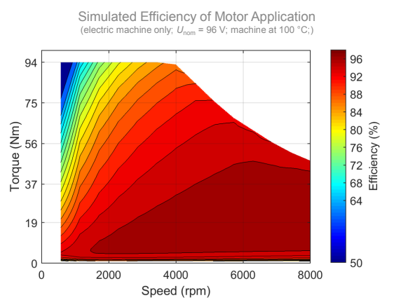 Note the performance at low revs with a high torque demand. It must be remembered that we are in competition and most of the time a high demand is made.
On the other hand, this motors are more elastic than thermal engines, so it doesn’t have much sense to install a gearbox with many gears. From the experience of other teams and editions, they only use the last two gears of a commercial gearbox.
As you can see on the performance graph of the electric motor used in the previous edition (Engiro), the efficiency of the electric motor at low revolutions is close to 50% meanwhile at high revolutions it can achieve 90%. This is a good reason to install a gearbox rather than to get more output torque.
Introducing a gearbox for racing has two handicaps:
- Shifting time: To get effective shifts on a gearbox, especially in acceleration, it needs to be fast shifting between gears, otherwise all the advantage can be lost there.
- Smoothness in shifting: Motorcycles are very sensitive to sudden movements. In fact, in competition, the goal of a gearbox is not only to be fast, it’s also to be smooth between shifts. This means, not generating strong impacts on the tire while shifting.
Of course, all this handicaps can be solved but it requires a big amount of testing and time. With this base, we manufactured a gearbox for the previous prototype:
 Render of the previous 3D unfinished prototype design.
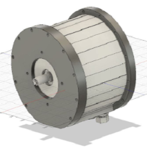
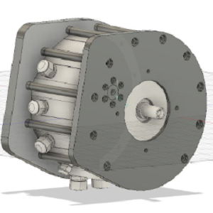
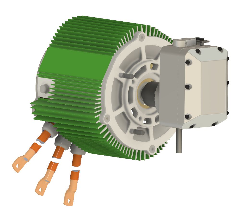 Electric motor and gearbox
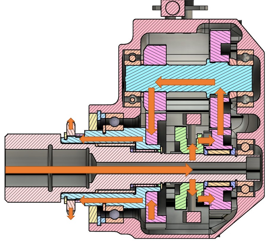
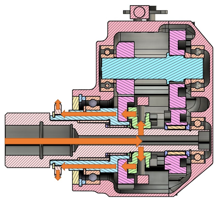
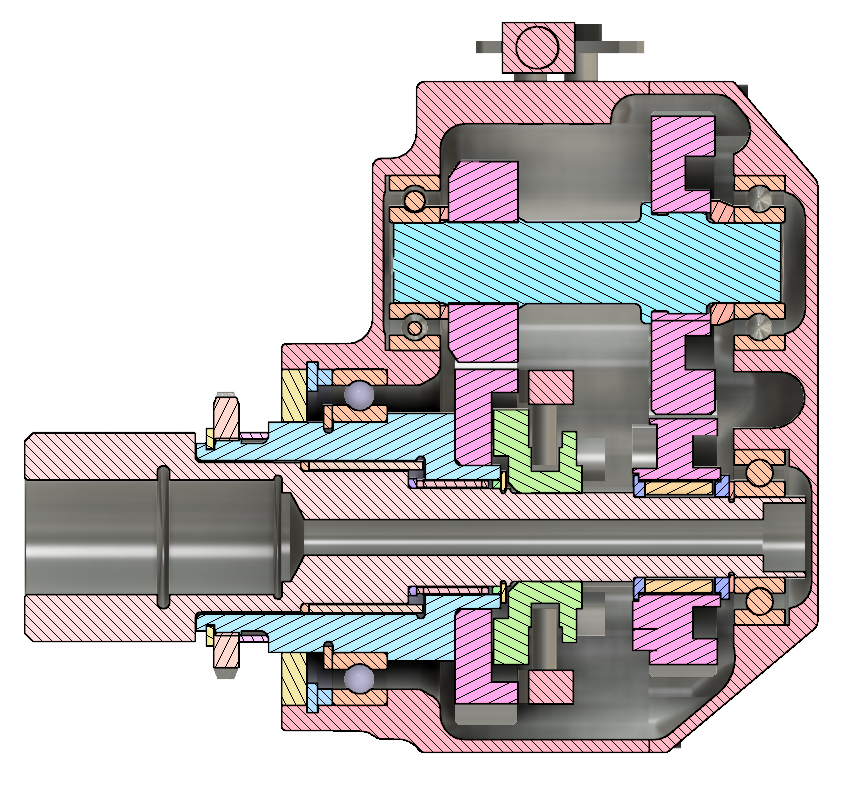 Section view of gearbox
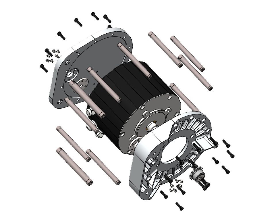
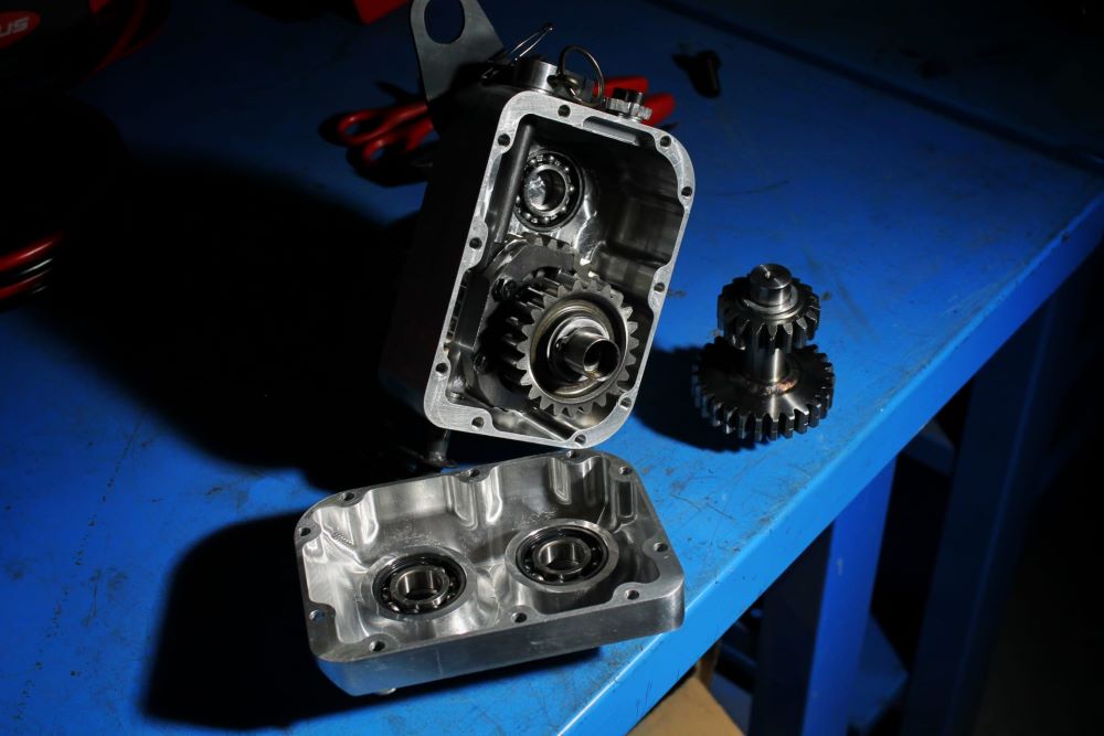 Gearbox details
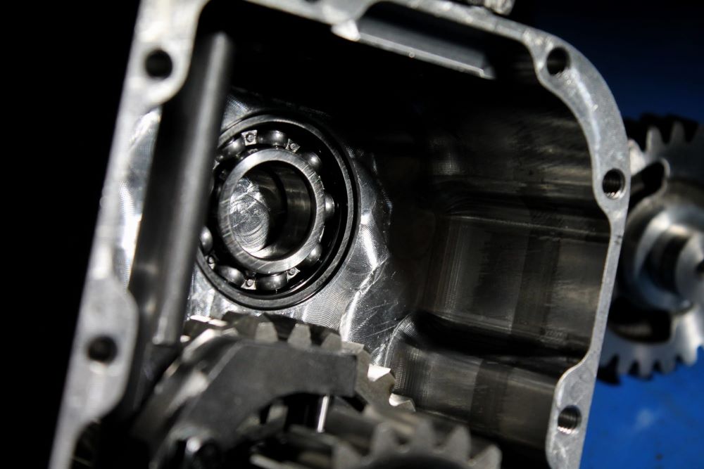 Gearbox details
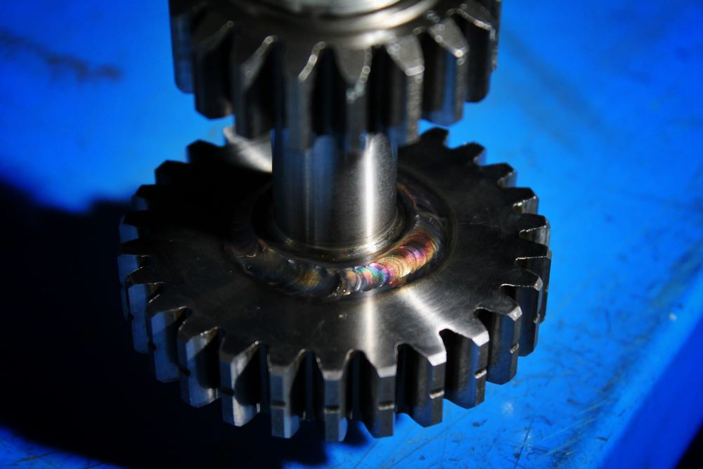 Gearbox secondary axis
This gearbox has two gears, one reduction gear and one direct.
 First gear
 Direct gear
We can see in the blue line the speed of the output shaft when we shift gears. In red, the revolutions of the input shaft.
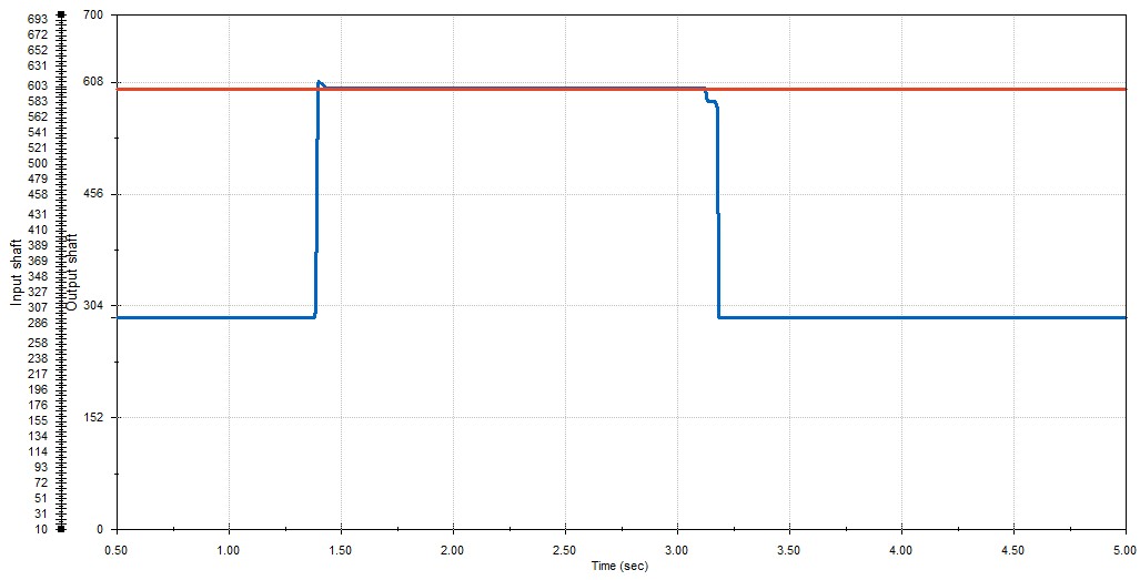 Gearbox simulation
After testing the gearbox we found two issues:
- The inverter was not ready to gear shifting: It’s not possible to program custom actions to make, for example a smooth shift. We found a workaround to solve this problem using a 0-torque power map to cut the power of the electric motor (like a quick shifter) but we didn’t have enough time to setup it correctly, so the rotor inertia caused a lot of knocks when shifting.
- Gear ratio: Gearbox normally have a small step between gears. The problem, as mentioned before, is that for an electric vehicle we need a big step between gears to make it worth having a gearbox (due to the elasticity of the electric motor). This causes a problem related with the previous one. When shifting, there is a big difference between the speed that the electric motor has and the speed that the electric motor should have on this new gear. If you can’t control this difference, the gears are going to knock when shifting.
These two issues make it complex to make it work in a short period of time and with a inverter that is not designed to support this features, we decided to discard this option for this edition.
Chain
As mentioned before, we are going to use a direct drive system with chain. There are multiple types of chains depending on the use and the force that they can hold.
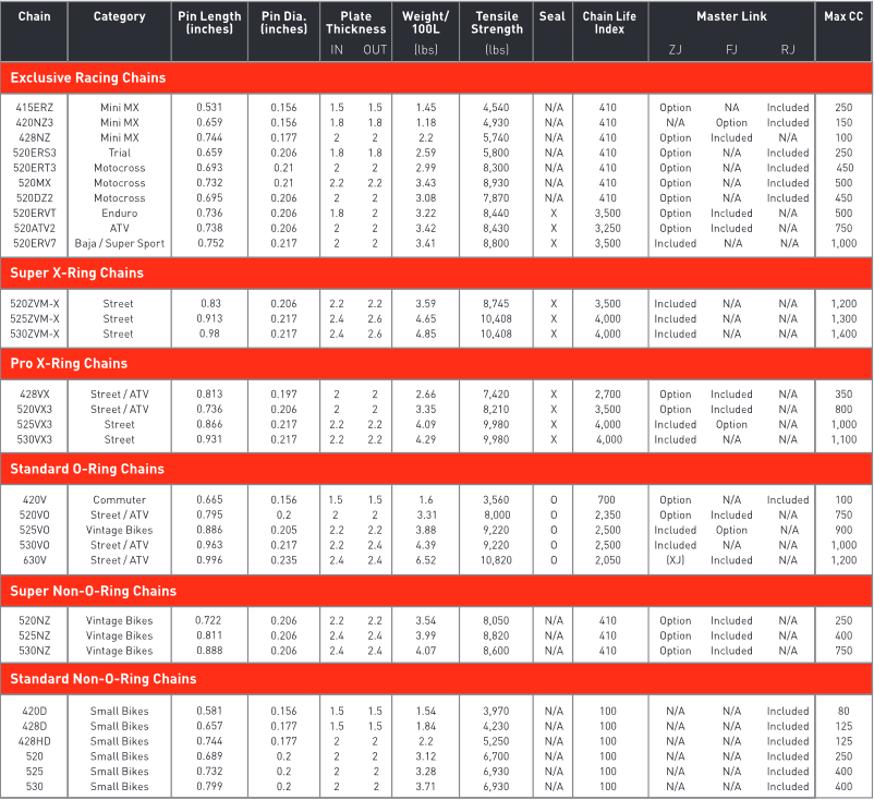 Source: DID motorcycle chains catalogue.7
After analyzing the torque that the chain should hold, a 415 it’s enough for the application. The problem was that the 415ERZ is a high quality chain and it’s expensive. We need to buy multiple chains to change the gear ratio for the different tests so this chain wasn’t an option. Instead, we choose a 428HD, it’s stronger than the 420 and cheaper than the 415 with similar specifications, a bit heavier but it was valid for us.
Final Design
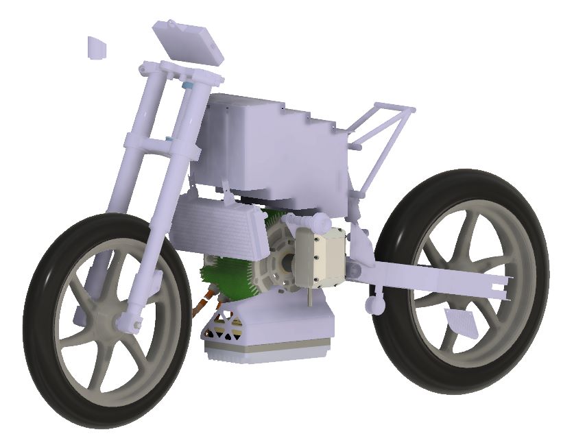
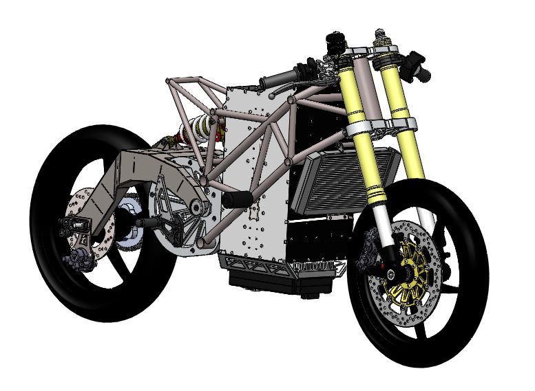 Mechanical 3D design
 Mechanical 3D design
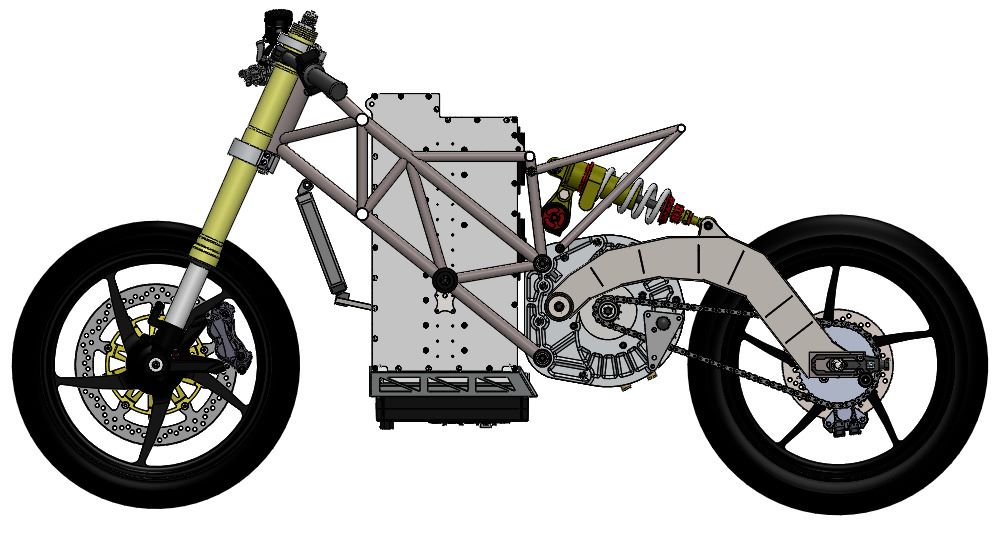 Mechanical 3D design
3D Software Comparison
Everything presented below is a personal opinion. During this development I had the opportunity to work mainly with two design software: Fusion360 and Solidworks. Some of the differences between this two software that I found during the design of the prototype are:
Fusion360
Pros
- Very fast initial learning curve. The menus and options are neat and clear.
- The PDM system offered by default is very simple and allows collaborative work storing all versions and being able to restore them as if it were a Git repository. In addition, while a user is working on a part or assembly, it is blocked for others avoiding problems.
- The graphical interface is very well designed, modern and clear. The sections of the parts are colored in such a way that each part is perfectly distinguishable.
- I have not tested it but the CAM module for milling must be quite powerful as I heard.
- It opens files from other software such as Catia or Solidworks.
Cons
- For simple assemblies it works well on any machine, it takes a while to start up but it is manageable. The problem comes when you start working with large and heavy assemblies. The increase of RAM usage is exponential and you need a machine with a lot of resources to be able to move it smoothly.
- Many of the options are in the cloud, such as finite element analysis. Personally I don’t like too much how it works.
- When working with assemblies and references between them, many times the references were lost. On the other hand, the contexts used to establish an assembly at a specific time when a part derives from it did not work well for me. I probably didn’t fully understand how it internally works.
- The joints in assemblies are all mechanical. You need to understand how they work to use them correctly and is not as intuitive as Solidworks.
Solidworks
Pros
- Very stable software.
- Moves large assemblies smoothly on a PC with fewer resources.
- Powerful add-ons are available to perform finite element and CFD analysis.
- The sheet metal module is complete.
Cons
- The initial learning curve is a bit harder than with Fusion360.
- It does not have a threading wizard as advanced as Fusion360.
- The 3DExperience PDM is very complete but more difficult to use than Fusion360 for a small project.
If I had to make a decision for a personal project I would consider the purpose. If it is a small project, for 3D printing or machining, Fusion360 would probably be the choice. For larger projects or large companies, I would choose Solidworks without any hesitation. It’s more expensive but perfect for that use cases.
Manufacturing and Assembly of the Components
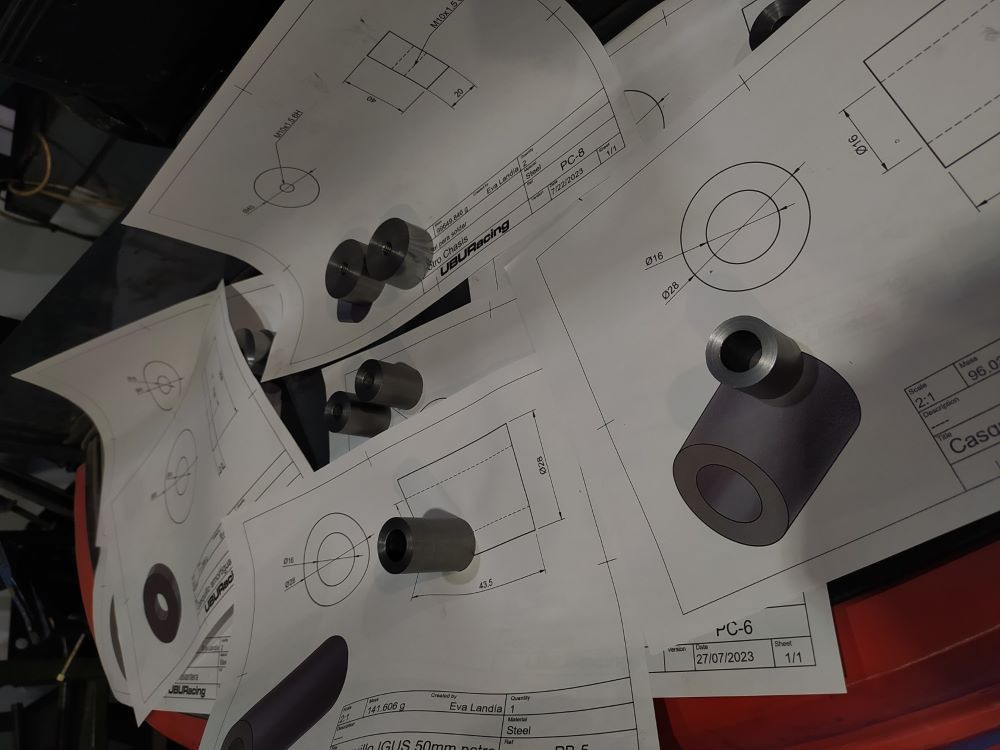
With the design finished, we started manufacturing all the parts for the prototype. We got help from the sponsors for some parts like laser cut and machining. Others were made by us. Of course to get this done we exported all the drawings to manufacture it.
 Example of manufacturing drawing
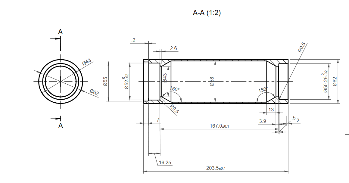 Example of manufacturing drawing
Chassis Manufacturing
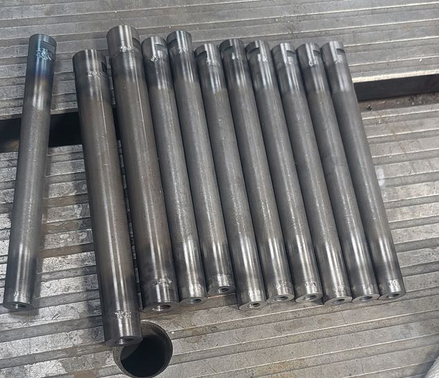
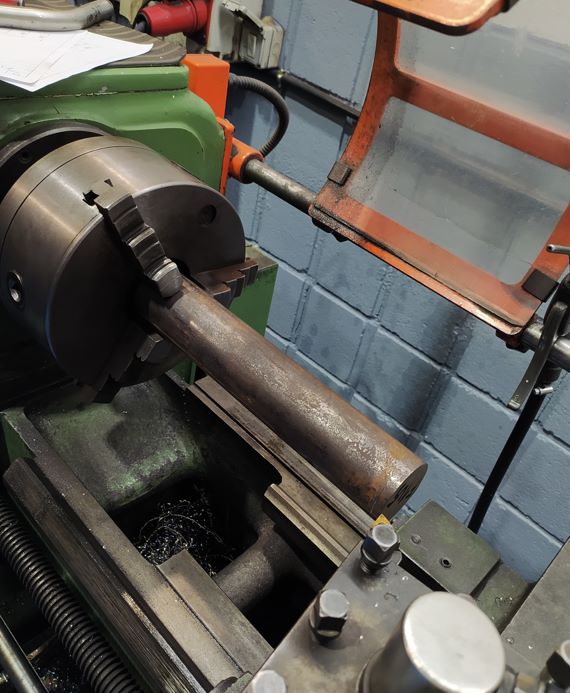
The chassis is mainly built with pipes, bushings and other mechanized parts. We got the pipes cut with laser from one of our sponsors and the rest was machined by me with a lathe and milling machine.
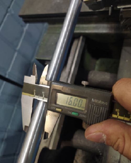 Starting from a raw bar, the outside is reduced to 16mm of diameter |
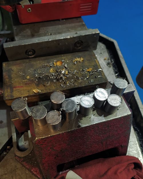 Cutting the bar for bushing manufacturing |
 Zero motorcycles motor position |
 Zero motorcycles swingarm. Output shaft and swingarm pivot are aligned. |
 Welded brushings to pipes
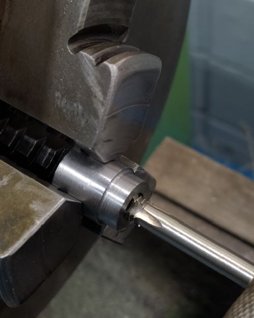
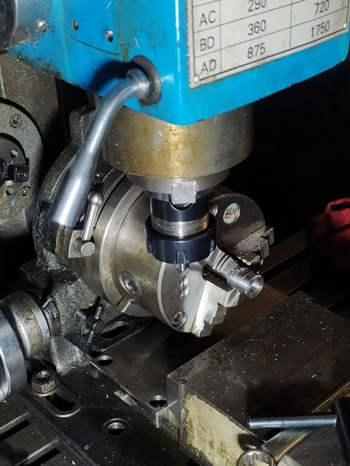 Machined to use a wrench to tighten the bolts to this pipes |
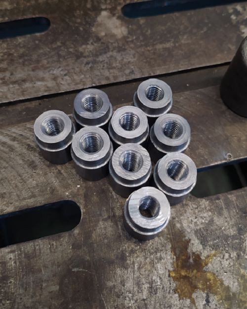
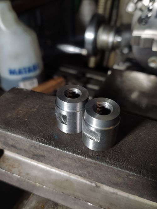 Finished bushings |
 Manufacturing of different bushings
 Lathe work
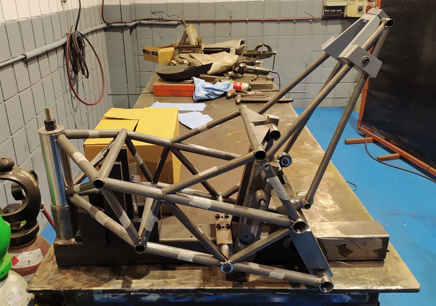
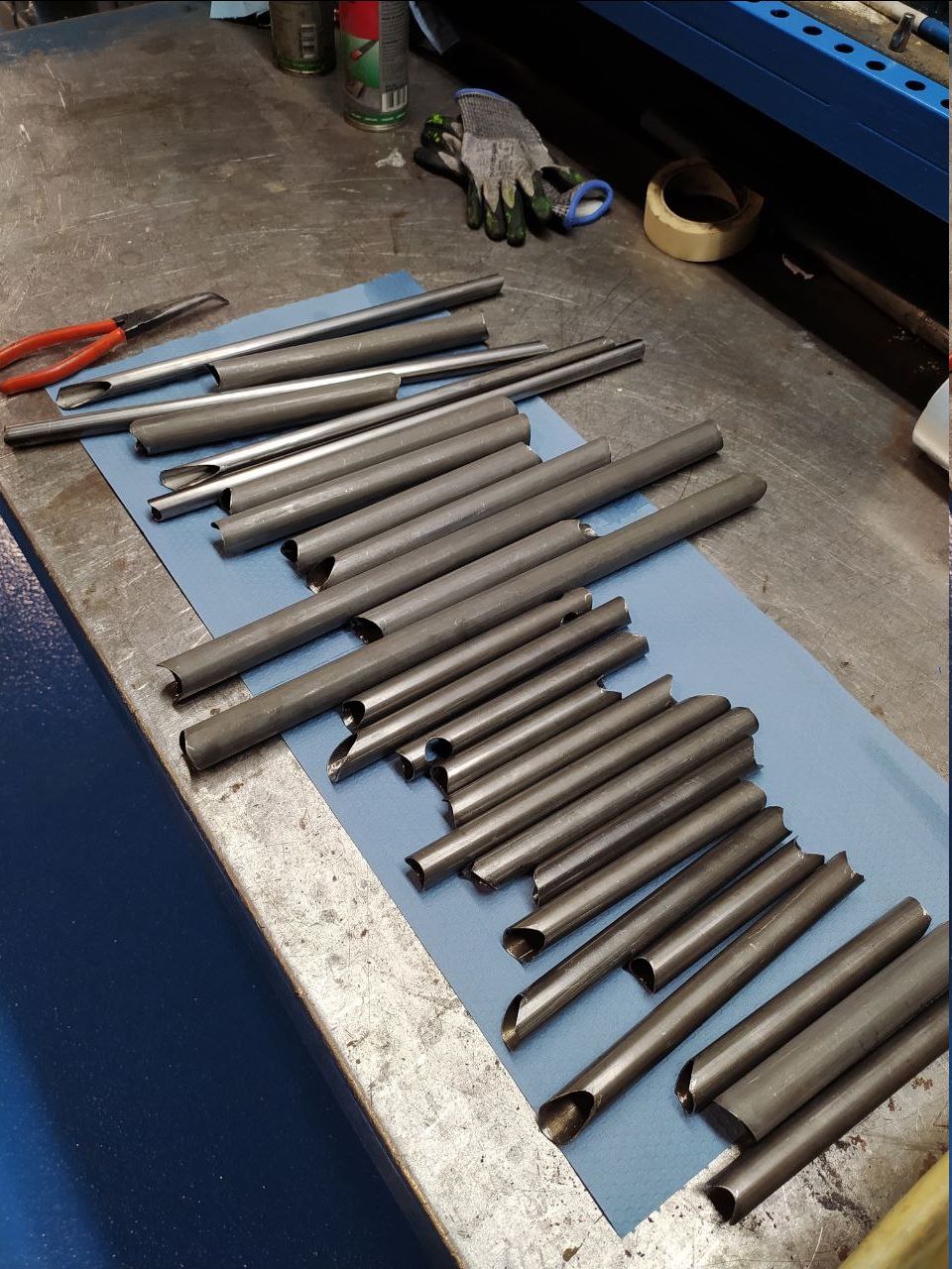 Laser cut chassis pipes.
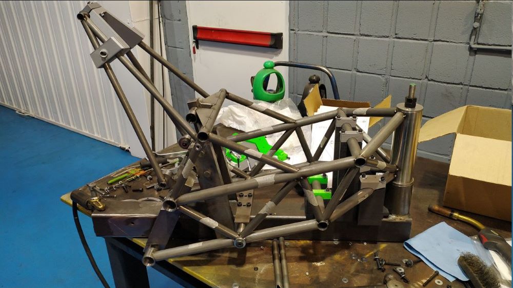 Initial welds on the chassis.
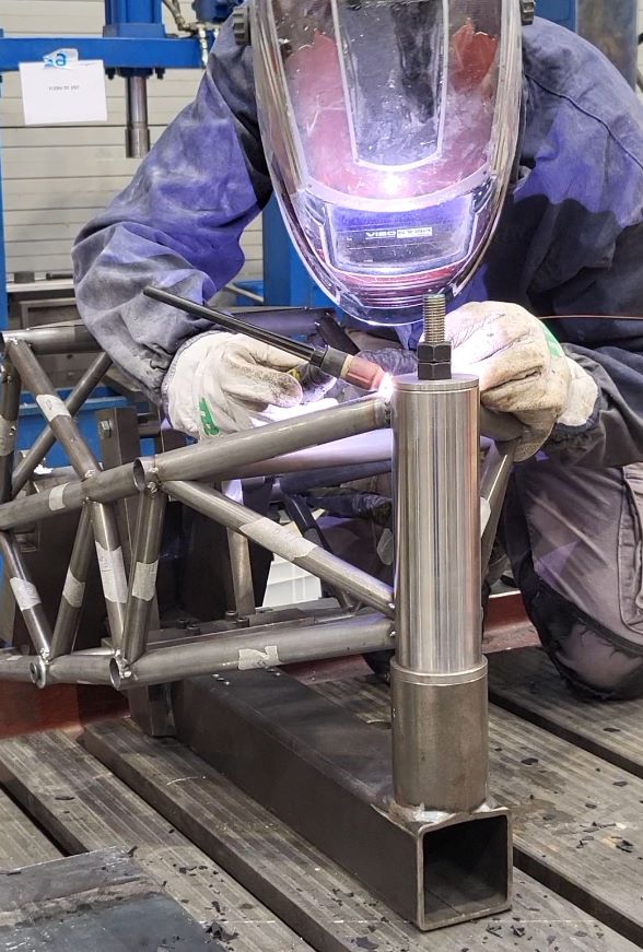 TIG welding process of the chassis. Note: We machined two bronze bushings to place in the bearing seat so that the diameter is not deformed during welding. In addition, this material will prevent the bushings from seizing.
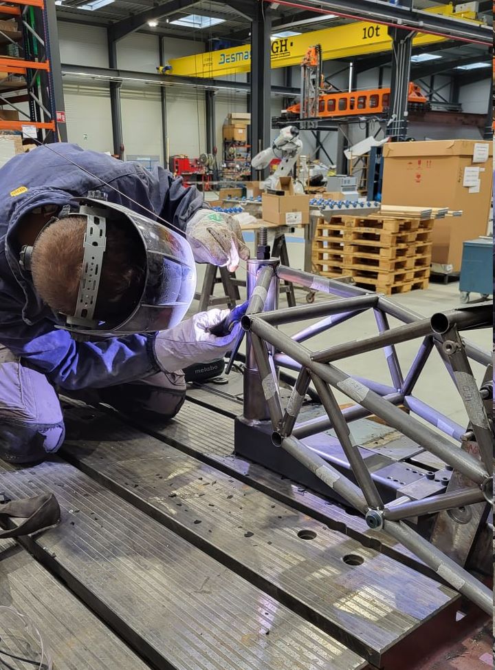 Chassis welding
Swingarm Manufacturing
 Brackets for rear axle tensioners. Brackets for rear axle tensioners. |
 Initial welding of the swingarm. Initial welding of the swingarm. |
 Swingarm parts Swingarm parts |
 Swingarm welding Swingarm welding |
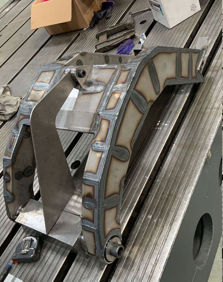 Welded swingarm
 Welded swingarm
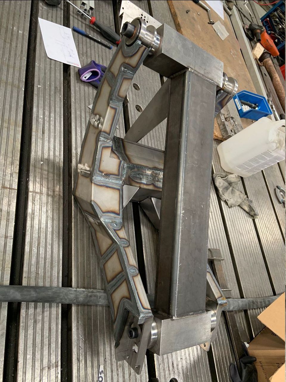 Lower view of the welded swingarm with the jig.
Final Assembly
 Chassis welding
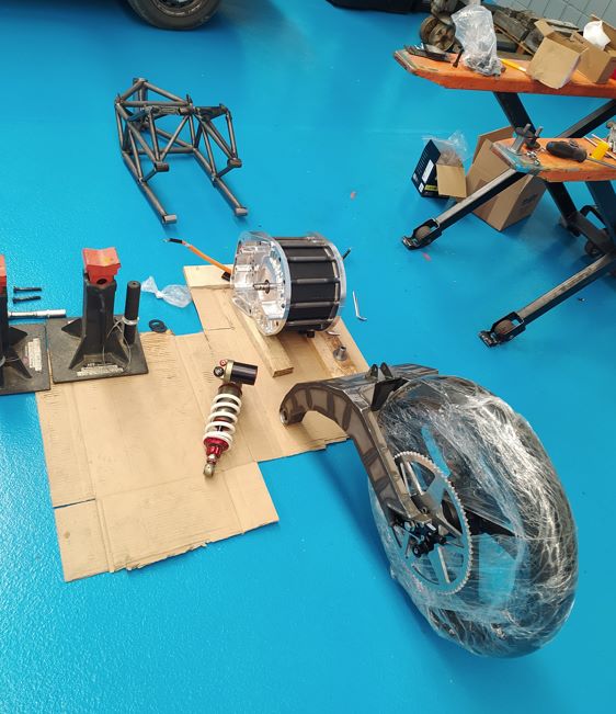
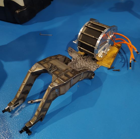 Swingarm and electric motor ready.
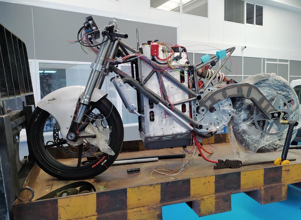
 Chassis, electric motor and swingarm ready.
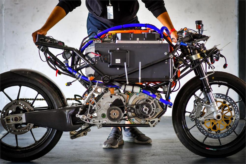
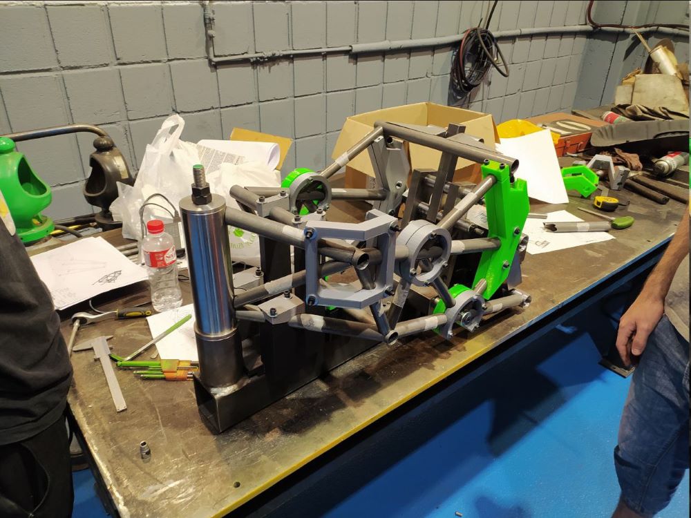
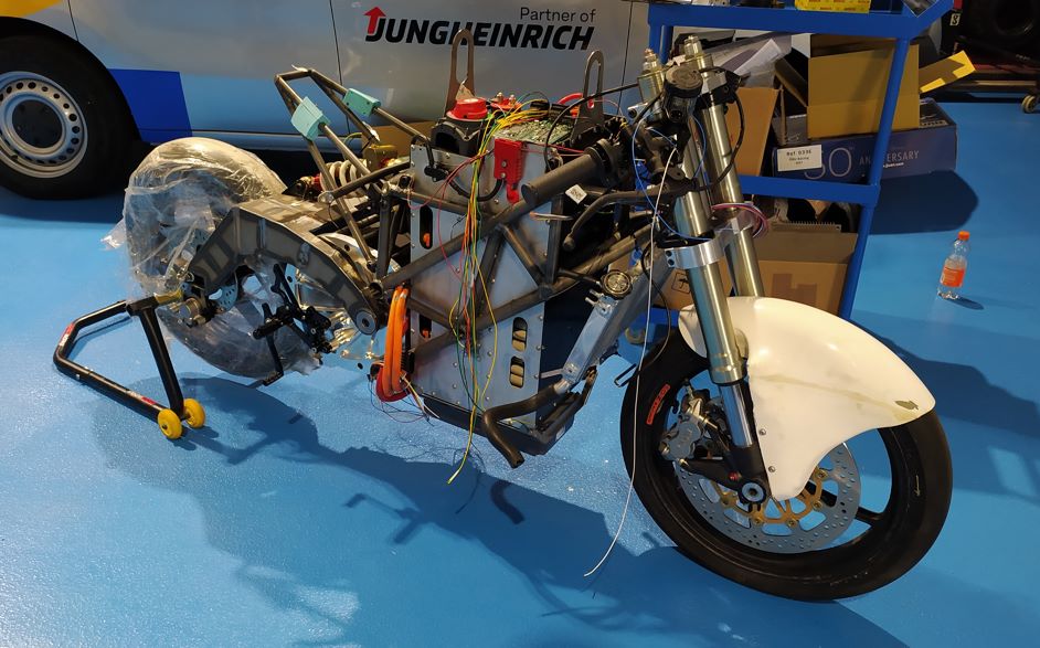
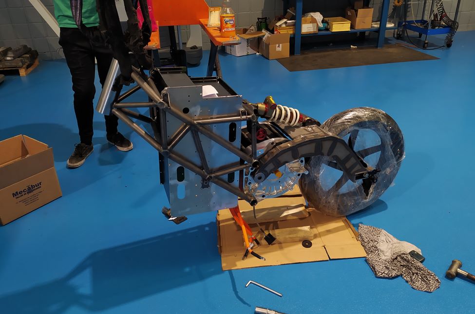 Pre-assembly
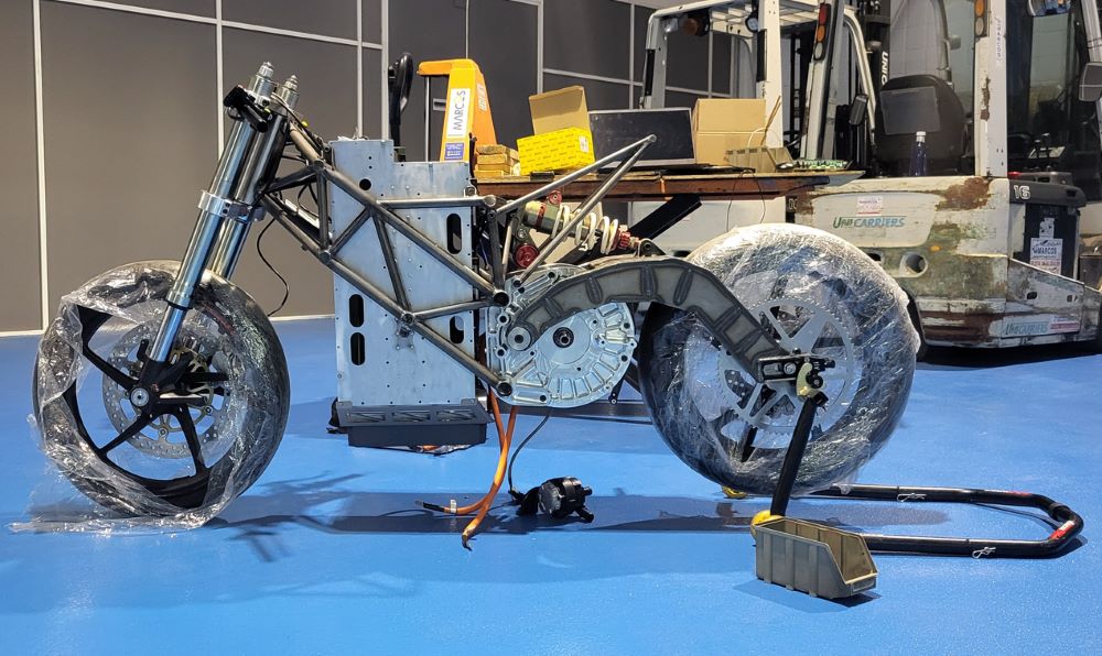 Pre-assembly. Note the empty battery
 Wiring electrical system
 Installing cooling system
 Finishing electrical wiring
 Forks out for adjustment
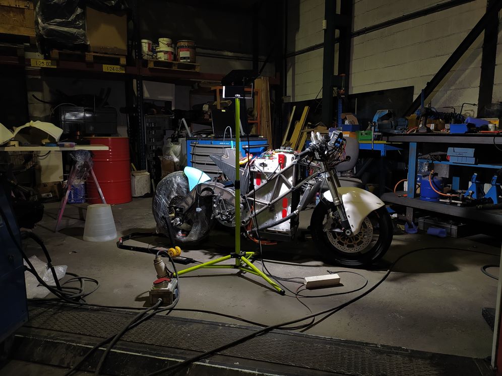
 Last test on the dyno before road testing
 Last test on the dyno before road testing
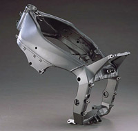
Fairing
For the fairing, our initial idea was to design and manufacture it completely by ourselves. For this it was necessary to manufacture molds (3D printed or machined in wood) and apply the material (fiberglass or carbon fiber) on them. Due to lack of time we could not make the fairing ourselves so we decided to buy one and adapt it to our prototype.
For this, due to the dimensions of the bike we decided to use a Moto2 fairing. In the previous edition we had used a fairing from Moto3 and the prototype was much smaller so we assumed that the Moto3 fairing would be too small for our current prototype.
It should be noted that the fairing of a Moto2 was big for this prototype too but there wasn’t middle size and we had no time to loose.
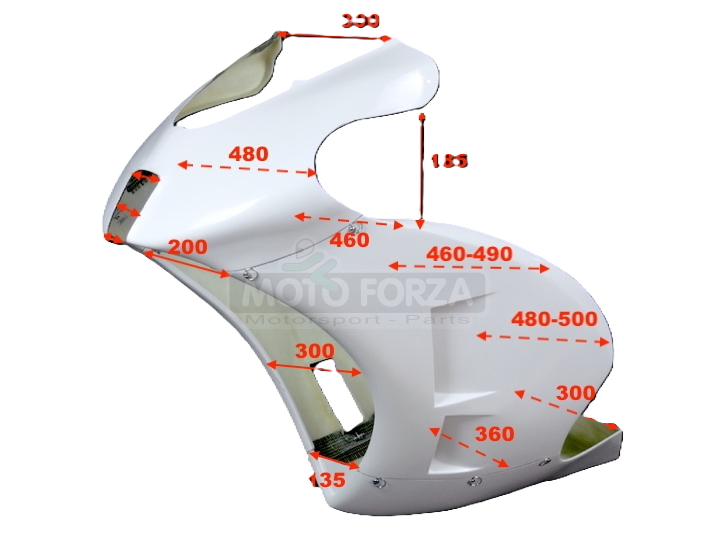
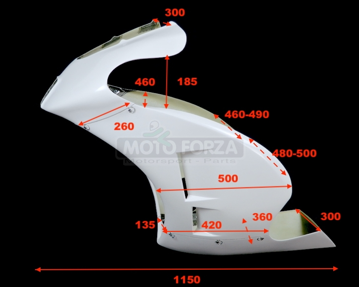
The process of adapting this fairing was artisanal, manufacturing brackets to hold it to the prototype. We had to open the keel because the inverter didn’t fit inside and close some air intakes that the fairing had and we didn’t need.
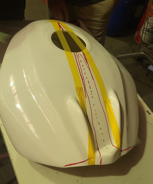 Cutting the tank cover to make it narrower
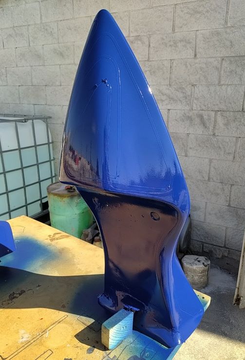 Painting the tail
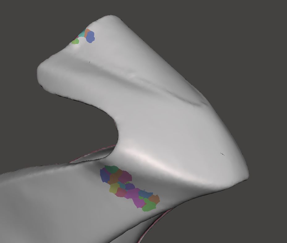
3D Scan
After manufacturing the fairing I would like to check on the CFD how efficient our fairing was. Also we needed it to create some gift for our sponsors so I scanned the fairing with a Revopoint 3D Range scanner.
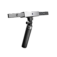 Revopoint Range 3D scanner
It’s surprisingly easy to use. You have to keep in mind that you need matte surface (you can sprinkle talcum powder) and be careful with dark and shiny areas. With the right lighting and surface conditions it works very well. After scanning it, you can get something like this:
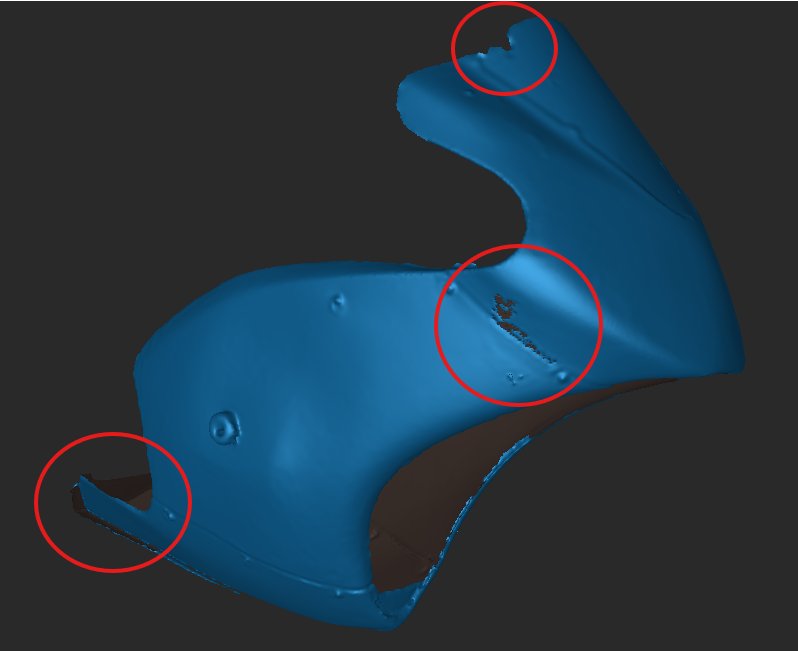 Result of the scan in Revo Scan 5 software
As you can see, the mesh is not perfect and it’s only one layer. We need to work on it to correct the issues and generate a solid body. We wanted to print it also on a SLS printer so surface is not valid for that purpose.
With Autodesk Meshmixer, we can edit the mesh. After a few hours, I got this:
 Body result in Meshmixer
This process was done with all fairing parts, the tail, tank cover and front mudguard. After that we got this result:
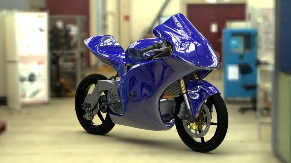 3D Render
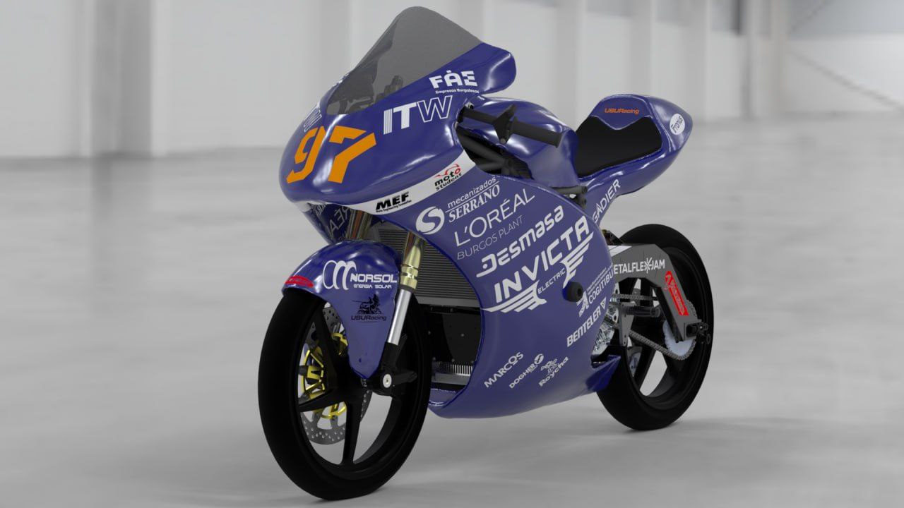 3D Render
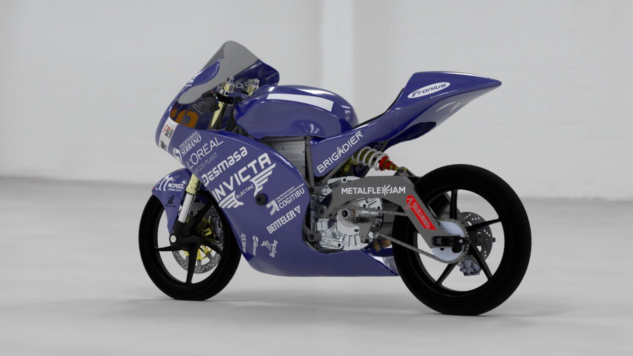 3D Render
FEA (Finite Element Analysis) & CFD (Computational Fluid Dynamics)
TO-DO
Result
Electronics ⚡
In this section, I will focus primarily on two topics: the vehicle’s electrical system and the telemetry, both of which we developed in-house.
Security Measures
One of the most critical aspects of an electric vehicle is its safety system. In our case, we use a battery with a peak voltage of 117V, capable of supplying 900A of continuous current with even higher peak outputs. The organization requires two main safety components to be installed: the IMD (Insulation Monitoring Device) and a safety circuit, which we’ll discuss later.
By regulation (and common sense), the vehicle has two separate electrical systems: HV (High Voltage) and LV (Low Voltage). In a conventional vehicle with a 12V battery, the chassis serves as ground, meaning the negative terminal is connected directly to the frame. However, in high-voltage vehicles, this approach is only partially applicable.
The high-voltage system is directly connected to the battery and must be a “floating” system, completely isolated from the vehicle chassis. This configuration requires two different grounds: one for the HV circuit and another one for the LV circuit. The HV ground should never come into contact with the chassis, whereas the LV ground is connected to the chassis, similar to a standard vehicle battery.
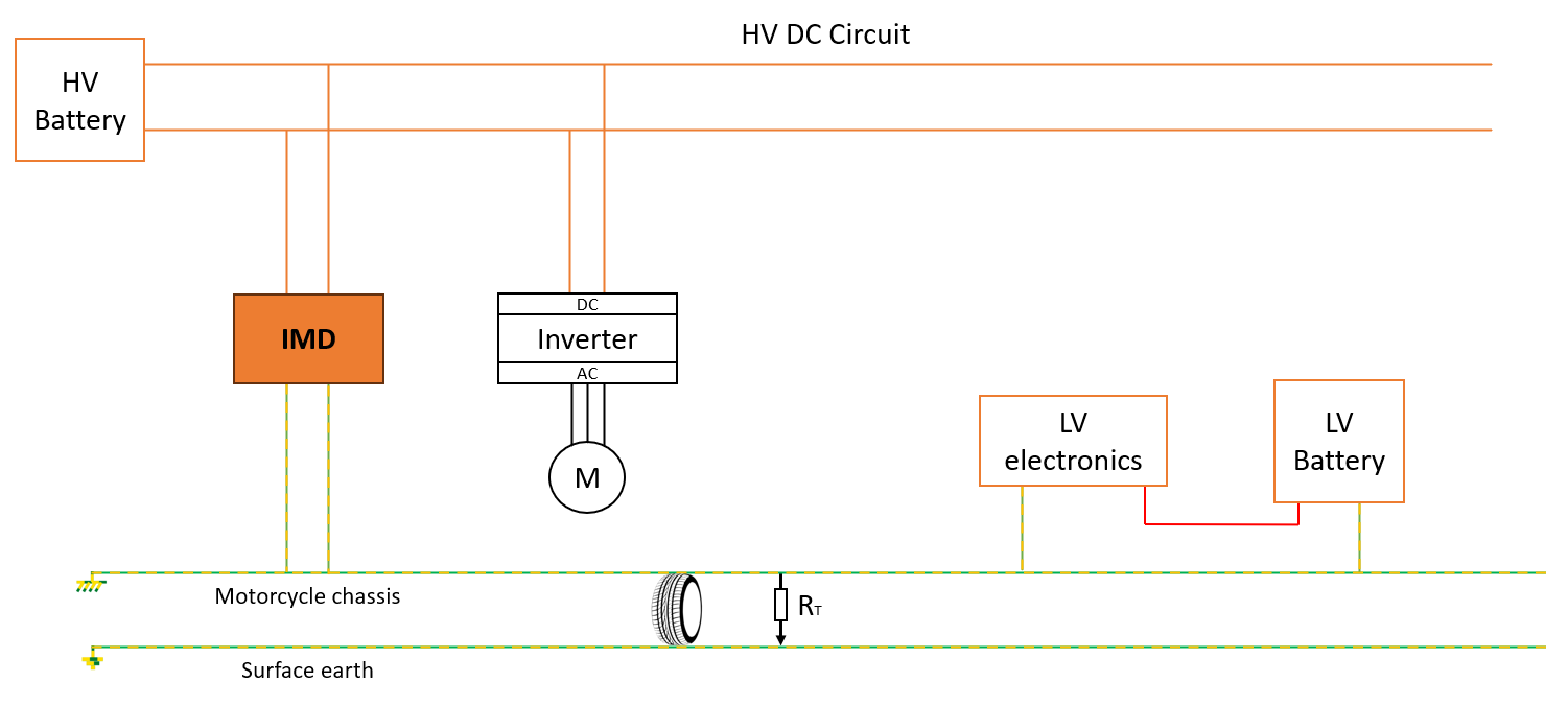 HV and LV systems
This configuration ensures that neither the rider nor anyone touching the vehicle will ever be exposed to the high-voltage system.
IMD (Insulation Monitoring Device)
Referring to the electrical diagram, we see an important component named IMD. This is an electric vehicle with both high-voltage and low-voltage systems, and one of them presents a potential safety hazard. An IMD (Insulation Monitoring Device) is required to monitor and protect against electrical faults.
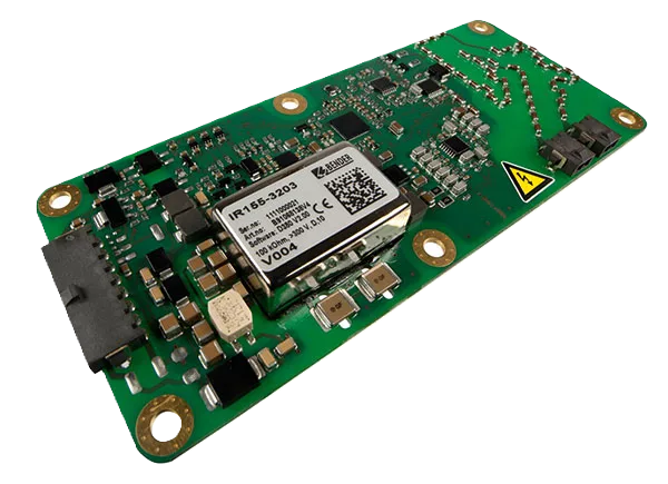 Organization’s IMD9
In simple terms, the IMD is similar to a differential circuit breaker in a traditional electrical installation. It’s connected to both, the HV and LV systems and can detect insulation faults between the two circuits, down to a resistance of 10 MΩ. This feature helps protect the rider or others from exposure to the HV circuit in the event of a fault.
The device setup is straightforward, as shown below:
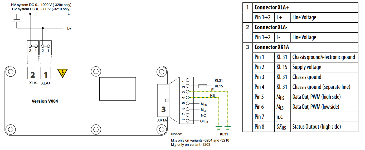 IMD pinout9
- XLA-: Negative line of the HV system (0 to 1000V).
- XLA+: Positive line of the HV system.
- Pin 1: Supply ground.
- Pin 2: Supply positive (12V or 24V).
- Pin 3: Chassis ground.
- Pin 4: Additional chassis ground connection.
- Pins 5-7: Unused.
- Pin 8: Status output, activated when insulation is intact, enabling or disabling HV power via the SSRelay.
With this information we can start working on the security circuit.
Security Circuit
For the security circuit, the organization offer us two options:
Disconnection system with contactor directly controlled by the disconnection circuit:
 Option 11
This is not our case so I will skip it.
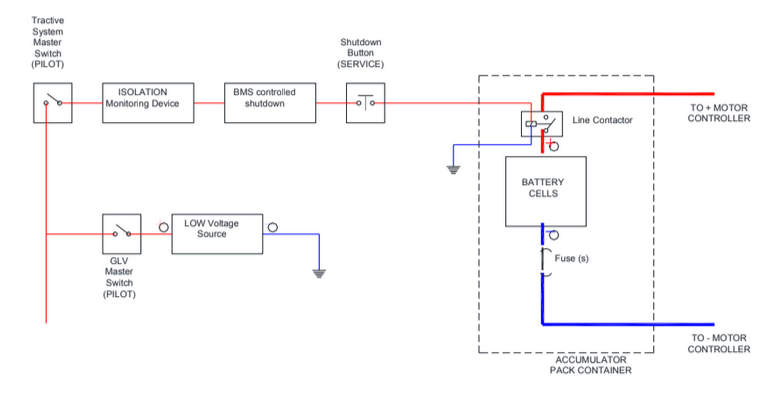
Disconnection system with contactor directly controlled by the controller:
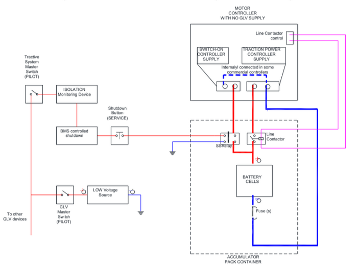 Option 21
This is the schematic we will use. Let’s focus on the right side of the diagram where we have the battery pack with high-voltage (HV) positive (red) and negative (blue) lines. The positive power line includes a line contactor positioned between the inverter and the battery, controlled by the inverter via pink wires. When the inverter is ready, it activates the line contactor, closing it and supplying power to the inverter.
This process occurs when the SSRelay is closed. The inverter has two positive lines: one is the power line, as explained earlier, and the other, connected through the SSRelay, is for the logic supply. This line also carries high voltage but at a very low current (around 5A for our inverter). When the SSRelay is closed, electricity flows from the battery pack to the logic supply, starting the inverter. Once the inverter is ready, it enables the line contactor control, closing the line contactor and initiating the inverter’s traction power.
The SSRelay is controlled by a low-voltage signal (12V in our case), acting as an interface between the high and low voltage circuits. To open or close the HV circuit, switches can be placed in series with the SSRelay control. If any of these switches are opened, the HV circuit will also open. For example, the IMD is connected in series with the SSRelay, so if there is an insulation issue between the HV and LV systems, the SSRelay will disconnect power from the inverter, causing the main contactor to open as well.
Wiring Architecture
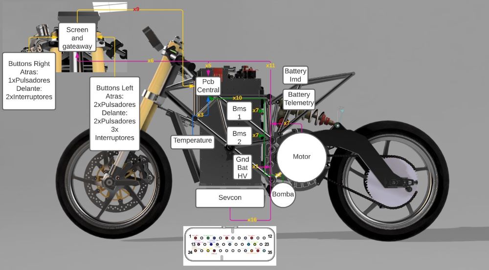 Wiring architecture
With the security system in place, we could begin working on the high-voltage (HV) system. Using the service manual for the Sevcon Gen4 Size6 inverter, we started designing the electrical scheme.
Inverter Scheme
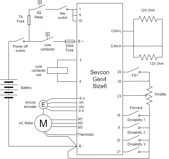 Sevcon Gen4 Size6 wiring
As we can see, it’s a simple schematic. Starting clockwise, we find two CAN-bus pins. These pins are used for the programming port and for monitoring. We created a CAN-bus network to collect all the data with our data logger, as I will explain later.
Next is the throttle input, which has a switch that activates or deactivates in the resting position for safety. The inverter can be configured with this switch as FS1, meaning it will not read the throttle potentiometer signal unless the switch is closed, preventing unintended acceleration.
Following that is the potentiometer, which ranges from 0 to 5k ohms. It has a positive input, a signal input, and a ground, which is shared with the battery’s negative terminal (B-).
Lastly, there are several switches. The “Forward” switch must be closed to enable the vehicle to start moving. The “Drivability 1, 2, and 3” switches allow for different maps and characteristics to be set, such as limiting speed or reducing power as requested.
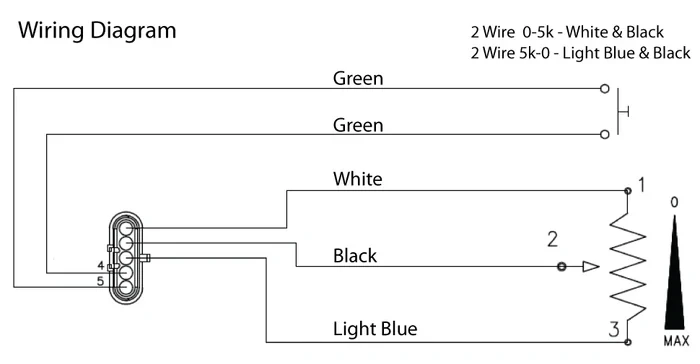 Domino twist grip throttle wiring diagram10
After that, we can see the electric motor. It has three power cables and another connector, typically for the thermistor, which measures the motor’s temperature, as well as the encoder signal. The encoder has four wires: positive, ground (different from B- and isolated), and the sine and cosine pins. This setup allows the inverter to determine the rotor’s position.
Next, there is the line contactor coil. This is driven by the inverter. When everything is ready, the contactor closes, and power is supplied to the inverter. In the middle of the line contactor, there is a manual disconnector that allows us to open the circuit even if the contactor remains closed for any reason, this is just for safety.
Finally, we have the key switch input. This inverter has three inputs for the same function because it has a high current consumption (a maximum of 7A), so we will connect all of them. In series, we have the SSRelay, which is driven by the LV circuit, as we will see later.
HV (High Voltage) Scheme
Let’s take a look at the HV scheme. We are using a 28s 20p battery configuration. This means that we have 28 series and 20 parallel cells. I will talk about this in more detail later, but to introduce the concept, with these lithium batteries, we need to control the voltage of all the series connections (monitoring the parallel connections is not necessary, as they automatically balance themselves).
This is where the BMS (Battery Management System) comes in. Once we had the battery designed, we needed to charge it. The problem was that we had a sponsor who could provide us with some battery chargers, but these did not reach the 117V we needed. To solve this, we chose to charge the battery in two parts, as shown in the image. The chargers we planned to use are isolated between the DC and AC sides, allowing us to work with them in parallel even if the HV is connected to the inverter. The only common point between them is the data logger, as we use the BMS to read the cell voltage and store it. This was accomplished with two isolated CAN transceivers, preventing short circuits.
The BMS is used “only” for charging. I say “only” because current flows through them only during charging. For discharge, we are connected directly to the positive and negative poles of the battery, but we continue to use data from the BMS to monitor the voltage of each module. If something goes wrong (such as significant module imbalances or has low voltage), we cut the power to the battery. I will discuss this further in the section on the charging system.
 HV scheme with battery detail
LV (Low Voltage) Scheme
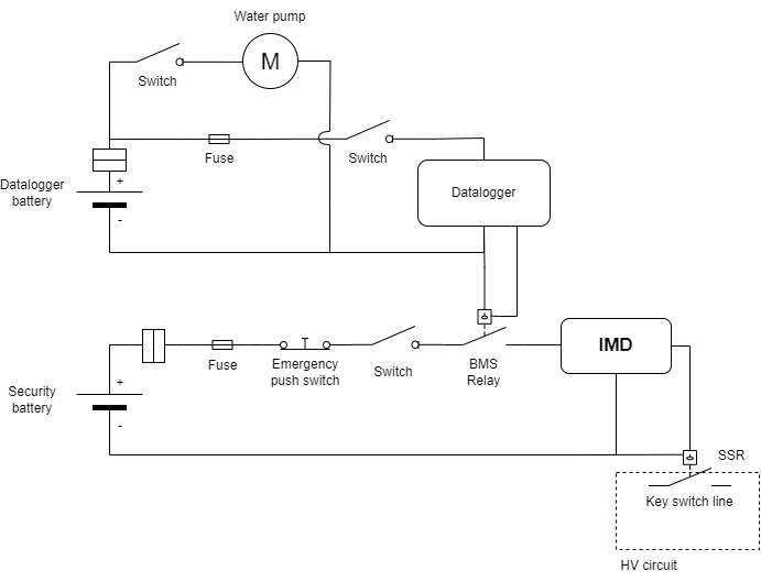 LV scheme
We have a simple electrical diagram with two batteries: one for the safety elements (IMD) and another for external components such as the data logger and the water pump. This setup provides a basic scheme for the operation of the prototype without mixing different functionalities.
As you can see, we have elements connected in series, including a fuse, an emergency button, the LV system switch, and the BMS relay. This relay is controlled by the BMS MCU. Next, we have the IMD, which will enable the output if everything is working correctly. This entire circuit manages the control part of an SSR (Solid State Relay).
Wiring Diagram
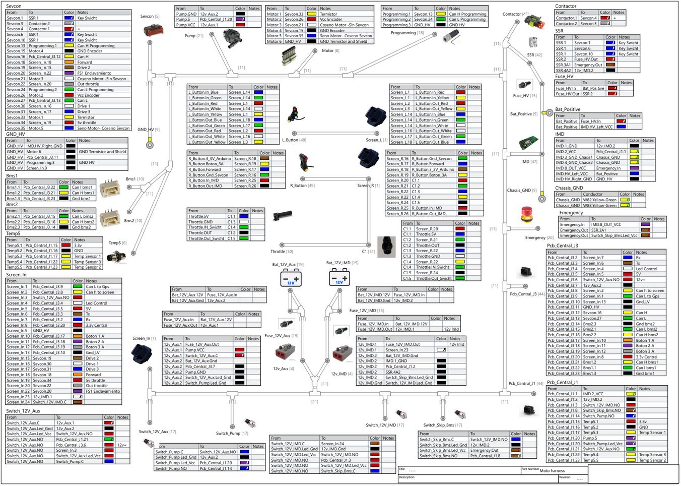 Electric elements and connections
Datalogger
The data logger is the system that collects data for later analysis. It allows us to know what has happened while the vehicle was running and when we had no physical access to it. This system will enable us to analyze the battery voltage, temperatures of various components, and many other signals.
We had two alternatives for this system: to purchase a commercial one or to design and manufacture one ourselves. From our perspective, it’s more interesting to develop and manufacture our own, as the goal of the project is to learn and experiment with these type of applications. That is why we decided to develop one ourselves.
Features
The main features we were looking for included:
- The ability to collect data in real time and store it for later analysis.
- Display important data to the rider on the dashboard.
- Implement safety controls for certain situations, such as low battery voltage or high temperature in any of the components.
In more detail, the characteristics with which we designed this system included:
Data collection and storage
-
Inverter:
- Voltage received by the inverter
- Current consumption
- Throttle position
- Selected power map
- Speed
- Motor temperature
- Inverter temperature
- Motor RPM
- Iq, Target Iq, and Id, Target Id currents
- Ud and Uq voltages
- Power status
- Forward status
-
BMS:
- Total battery voltage
- Individual cell voltage
- BMS data
-
Sensors:
- Battery temperature sensors
- Radiator water temperature sensor
- ADC of LV system batteries
- IMU (Inertial Measurement Unit)
- GPS position
Dashboard data:
- Battery status
- Speed
- Selected power map
- Motor RPM
- Temperatures
- Data logger status (Recording or stopped)
- Power status
Safety
If a battery module falls below a certain voltage, if there is a highly unbalanced module, or if one of the modules reaches a high temperature, the high voltage system of the prototype will be cut off.
Datalogger Scheme
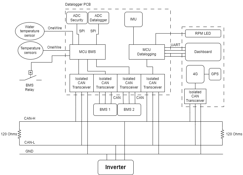 Architecture of the datalogger system
Mainly, as you can see, we have two MCUs. This was due to two reasons:
- The DUE MCU only has two CAN controllers, but we needed three (two for the BMSs and one for the inverter).
- We required a fast response for some features, such as the data logger, while other features, like BMS voltages and temperature sensors, could operate at a slower pace. The library for the OneWire protocol is blocking and slow, and we didn’t have time to program it again.
Of course, there were many better options, such as using a second smaller microcontroller, making RAW requests to the temperature sensors, and more, but we didn’t have time, and we needed something that would work on the first try. Also, polling is not the best methodology, we should have used interrupts to avoid blocking functions during firmware execution, but we programmed all of these features in just a few hours.
Components
The data logger includes the following modules:
- DC regulator from 12V to 5V
- MCU for data logging (Arduino DUE)
- MCU for battery management (Arduino DUE)
- MicroSD slot
- IMU (Inertial Measurement Unit) (MPU6050)
- One isolated CAN transceiver for BMS1 (ADM3053BRWZ)
- One isolated CAN transceiver for BMS2 (ADM3053BRWZ)
- One isolated CAN transceiver for the inverter CAN network from the data logger MCU (ADM3053BRWZ)
- One isolated CAN transceiver for the inverter CAN network from the BMS MCU
- Level shifter for the dashboard (the screen operates at 5V) (TXB0106PWR)
- Isolated ADC (Analog-to-Digital Converter) for the auxiliary battery (MAX22530AWE)
- Isolated ADC (Analog-to-Digital Converter) for the LV battery (MAX22530AWE)
- Solid State Relay to enable BMS1
- Solid State Relay to enable BMS2
- Solid State Relay to enable the water pump
- Solid State Relay to cut the HV system
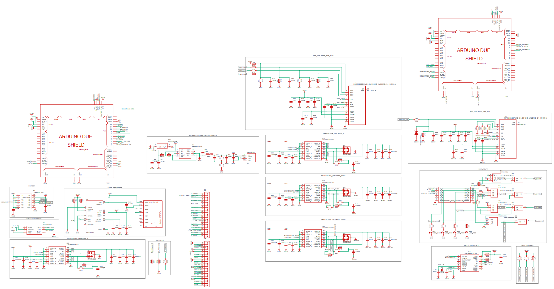 Board scheme
Hardware Design
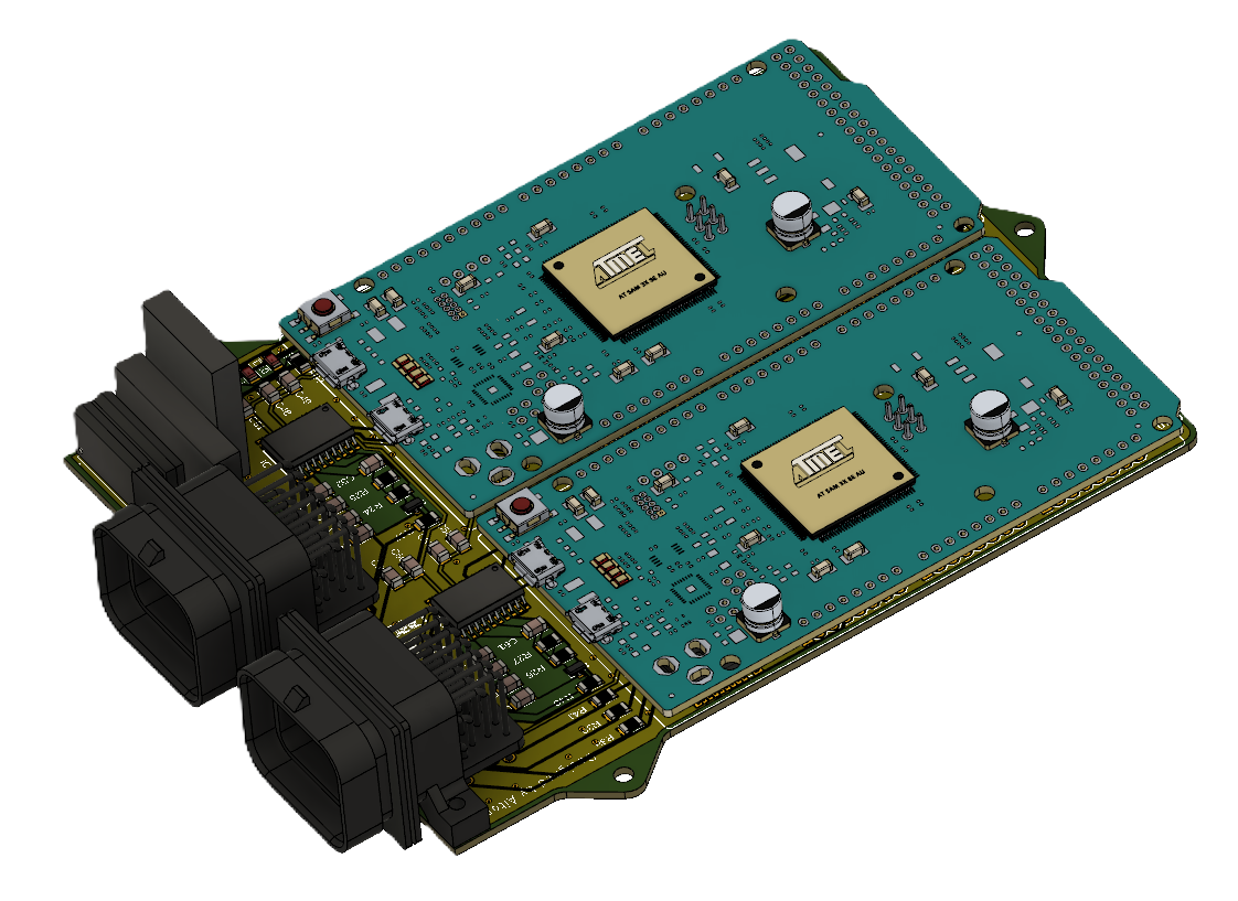 Upside view
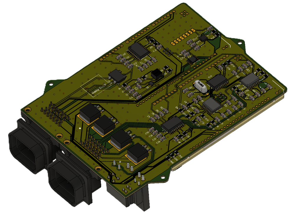 Bottom view
Screen PCB
The prototype had electronics located in different areas, such as the right handlebar, left handlebar, and central dashboard position, among others. We had two architectural options:
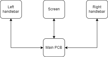 Option 1: Carry wire to all elements |
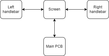 Option 2: Make a hub on the screen to connect everything |
The second option is more complex to design initially, but it is cleaner and more modular. If we need to disconnect one of the elements, we can do so without affecting the system. Therefore, we designed this PCB for that purpose:
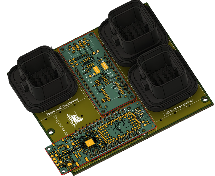 Upside view
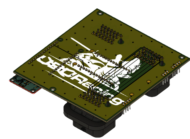 Bottom view
We also located two other boards here: one for GPS data and another for 4G telemetry. The GPS module will send data through the main CAN network, while the 4G module will retrieve this data from the CAN network to send it to a server. Unfortunately, we didn’t have enough time to finish this board, and it’s also not allowed in the competition to have a remote telemetry system, so we did not complete it.
As you can see, this board has three connectors: one coming from the main board and two for the right and left sides of the handlebar. On the right side, we had the throttle and three buttons for starting and stopping the electronics. On the left side, we had buttons to select different power maps and to start and stop data logging.
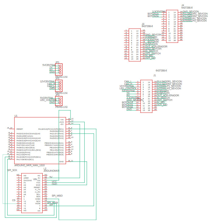 PCB scheme
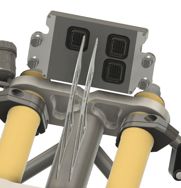 Connector view
Dashboard
For the dashboard, I used a Nextion screen. This screen has an embedded microcontroller, so you don’t need to send all the information continuously to the display. It has its own firmware with all the data needed to show the design, and you can connect through UART to send instructions to modify the elements.
For example, you have a textbox that can display a number. This textbox has a unique ID, and through UART, you can set the text by sending, for example:
textNumber.val=1 followed by three null bytes at the end.
We primarily had two screens: one general dashboard and another that provides information about all the battery modules for quick checking.
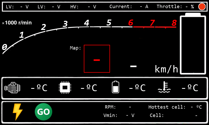 Main screen
On the main screen, we have some basic information displayed, such as:
At the top:
- Low voltage system battery level
- Secondary low voltage system battery level
- High battery voltage level
- Actual current used by the inverter
- Throttle position
- A red circle to indicate whether the data logger is recording data or not
In the middle:
- Electric motor revolutions
- Selected power map
- Speed
- HV battery level
- Electric motor temperature
- Inverter temperature
- Average battery temperature
- Coolant temperature
At the bottom:
- Connected/disconnected high voltage circuit
- Forward (throttle enabled)
- Maximum RPM achieved (for quick checking)
- Hottest battery module
- Minimum voltage module
- Position of the minimum voltage module
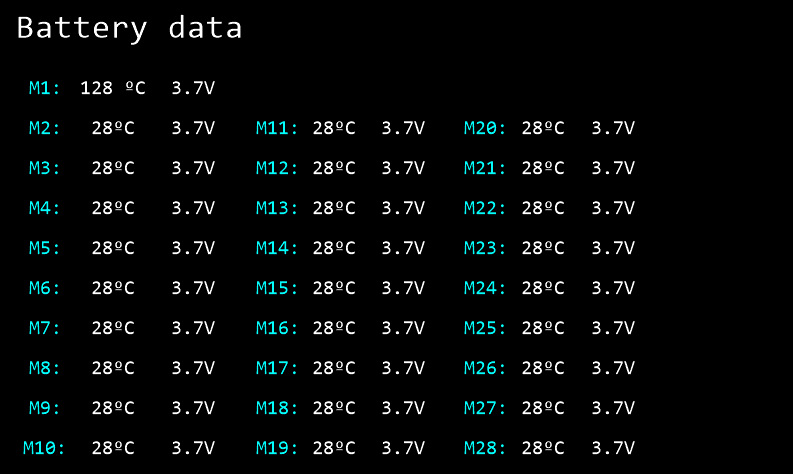 Battery information (module voltage and temperature)
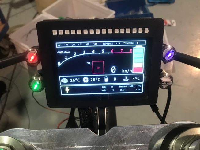 Working dashboard
Software Flow
Here is the simplified flowchart of the software logic. As explained before, we have two MCUs that are interconnected through the CAN network, so they have different logics.
BMS MCU
As we can see in the chart, it starts with the basic setup() function to initialize all the peripherals. The CAN interfaces are initialized by setting the connection mode and speed. Additionally, the OneWire interfaces are initialized. This interface is used to collect information from temperature sensors. We are using 28 temperature sensors with only three wires: positive, GND, and data.
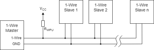 Example of OneWire topology.
The library for this protocol locks the MCU while retrieving the data, which is one reason why we used two MCUs (I know it’s not the best option)
With the interfaces ready, the MCU starts listening for CAN packets. Remember that we have three CAN networks: the main one that is connected to the inverter and the other MCU and two networks for both BMS. In this section, we are reading data from the two BMS networks to collect information about the battery status, such as module voltages and half of the battery voltages.
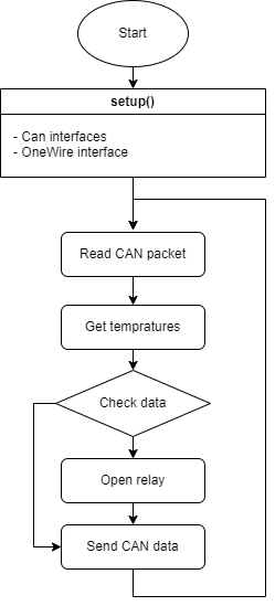 Simplified BMS firmware flow
With this data, the MCU requests the temperature from the sensors and collects it. If something unusual occurs (such as high temperatures, a significant difference between values, low voltages, or differing voltages between modules), the MCU opens the relay. This relay will turn off the power to the LV system, which in turn will cut off the power to the HV system.
After that, the collected data (temperatures and voltages) are sent to the main CAN network to be collected by the data logger MCU.
Datalogger MCU
This is the simplified flow of execution for the main MCU. First, the interfaces are initialized. Here, we only use one CAN interface to connect to the inverter CAN network. Next, the UART interface is initialized, and the screen is configured. The MicroSD card is also initialized with the input pins (for example, there is a button used to start/stop data recording).
Then, it starts listening for new CAN packets. When a packet arrives, it’s parsed and information is extracted. If it contains new data (different from the previous data) and data recording is enabled, this data is stored on the MicroSD card. If data recording is disabled, the information is only updated on the screen.
After that, the MCU checks for input changes (for example, if the data recording button has changed) and executes the necessary functions.
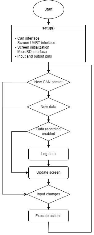 Simplified firmware flow
As you can see, the flowchart is quite simple. Of course, it has some tricky features, and setting up all these components for the first time takes some time, but in general, it’s not a complex flow for the basic functionalities that we wanted.
Manufacturing
With the gerber files exported, we ordered the PCB from JLCPCB. When it arrived, I started soldering all the components. After a few hours, this was the result:
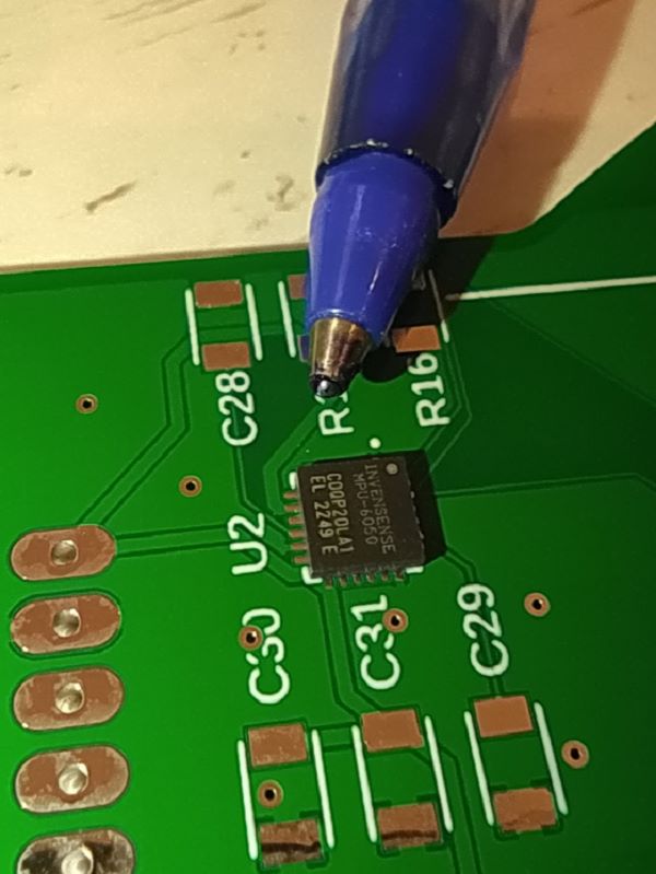 MPU6050 before soldering |
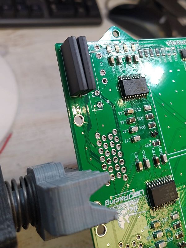 Soldering process |
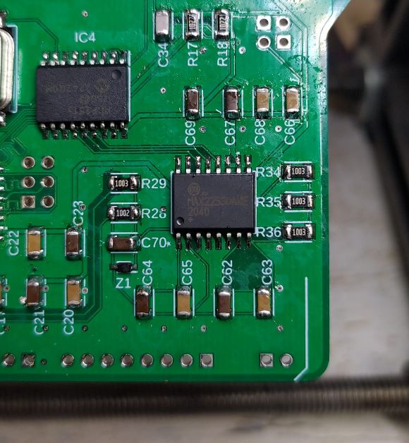 Soldering process
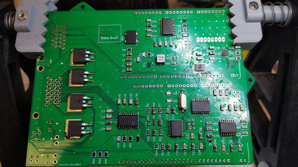 Finished PCB soldering.
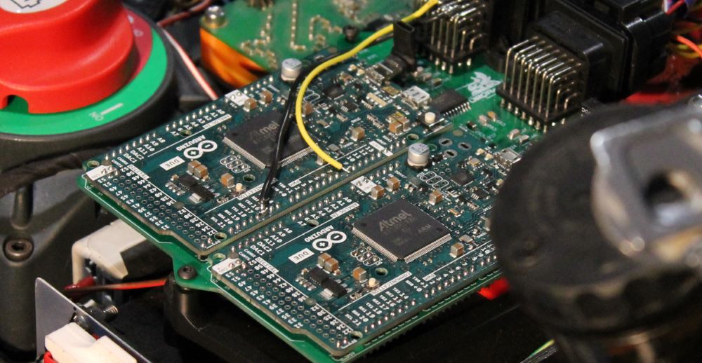 Electronics mounted on the prototype. We added two inputs to the connector for additional features.
Battery 🔋
One of the most important elements in an electric vehicle is the battery. It’s the component that takes the most significant volume, weight, and cost of the prototype. The battery was completely designed and manufactured by us. First, let’s take a brief introduction to batteries.
Introduction to lithium batteries
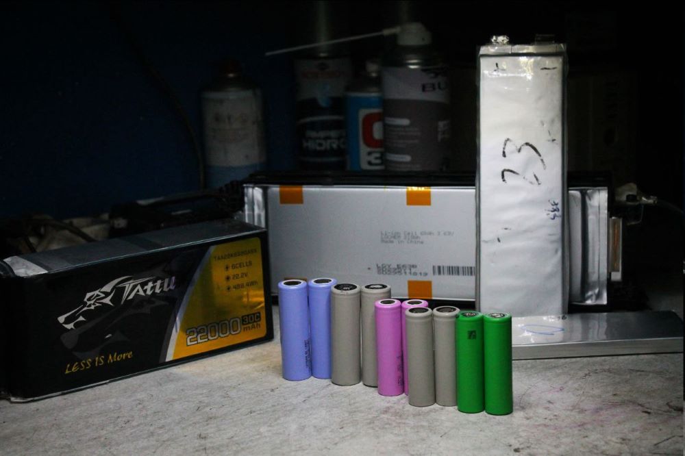 Different types of battery cell formats and technologies
Based on the number of cells we build our battery with, it will have greater capacity and power. We can mount the cells in two ways:
-
Series: By grouping the cells in this way, we achieve a higher battery voltage. In this arrangement, it is very important to note something about lithium batteries: we need to control the voltage of each cell individually. This is because not all cells have the same internal resistance, so some cells will charge/discharge before others. This situation is known as an unbalanced battery. To control this, there are devices called BMS (Battery Management Systems), as we will see later.
-
Parallel: In this configuration, we will achieve a higher battery capacity, meaning we can use it for a longer time or demand a higher current. It is important to note that cells in parallel function like a single cell with a higher capacity. In this setup, it’s not necessary to have a BMS, as the set of cells in parallel will self-balance.
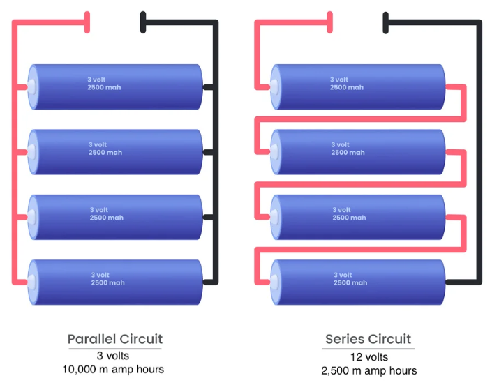 Parallel vs series connection11
We can build a battery using both connections. For example, a 24s 2p battery means that it has 24 cells in series and 2 cells in parallel.
Regarding the working voltage, it depends on the technology used to manufacture the cells, as we will see later. In our case, the selected batteries work within a voltage range of 4.2V to 2.5V. This means that in the example above, a 24s battery will have a voltage between 100.8V and 60V.
When discussing cell capacity, there is usually a relationship between the energy density and the discharge capacity of a battery cell. We will address this later, but for now, we just need to know that if we want to increase the capacity, we need to add more cells in parallel.
We must keep in mind that a battery will be limited by the series with the least capacity, so the battery should have a “square” structure. By this, I mean that if the battery is 24s 2p, each series must have 2 cells in parallel. If one of these cells in parallel fails or is not connected, the battery will have reduced capacity (limited to the series with only one cell). We also need to consider that this will require more current from that cell, which can be dangerous.
On the other hand, we have two different approaches when it comes to cell size. We can build the battery with many small cells or a few large cells. The advantage of using small cells is that we have a lot of modularity, allowing us to increase or decrease capacity in small increments. The disadvantage is that having too many cells increases the complexity of manufacturing and the possibility of failures (such as a poor weld connection, for example).
However, we need to find a middle point because if the cells are too large, we lose the modularity mentioned above. If we remove one cell, the battery can become too small, and if we add one cell, the battery can become oversized. For example, if you have a 24s 2p battery and want to upgrade it to a 24s 3p, you need to add another 24 cells, and if this cells are big, the battery will increase it’s size too much.
Additionally, as we will also see later, in general, the larger and higher capacity a cell is, the lower the supported discharge rate.
Battery Lifespan
One important aspect to consider in lithium batteries is their useful life. This is typically defined by the number of charge and discharge cycles they can withstand.
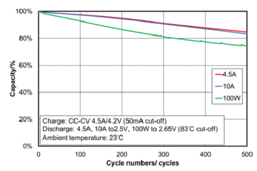 Example of cell capacity vs the cycles |
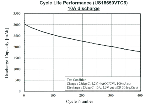 Example of Sony VTC6 cycles vs capacity |
The total number of cycles or the percentage of capacity loss in each cycle can be influenced by how the battery is treated. This includes the temperatures it has been exposed to, the demanded current, and how long it has been under “extreme” conditions.
For instance, a battery that operates close to its maximum temperature range won’t last as long as one that operates within an adequate temperature range. Similarly, charging and discharging up to the maximum and minimum voltage levels (such as 4.2V and 2.5V, respectively) reduces the battery’s lifespan. For this reason, many batteries used in vehicles don’t use their full working voltage range, trying to extend their useful life. However, in our case, we are prioritizing maximum performance and trying to extract the highest possible capacity in the smallest space. Therefore, we will push the battery to its limits, even if it reduces its life. Since the battery won’t be subjected to excessive use, we are far from reaching the cycles where significant capacity loss begins.
With all this information, our battery needs to meet the following requirements:
- Maximum voltage: According to regulations, the prototype’s battery cannot exceed 126V. However, the inverter we are using only supports up to 120V, which will be our voltage limit.
- Energy density: We need the battery to store as much energy as possible in the smallest space and with the lowest weight.
- Discharge capacity: As we will analyze further, the battery needs to be discharged in about 10-12 minutes, and not all battery types can meet this requirement.
Battery Technologies
The first thing to decide is which type of battery to use. Two main technologies need to be considered (although others exist):
- Lead-acid batteries: These are not suitable for our project due to their excessive weight and volume, making them impractical for our application.
- Lithium batteries: There are several types of lithium batteries, and they offer the highest energy density, making them ideal for this project. A few key technologies include:
- LiFePo4 (Lithium Iron Phosphate): Known for being very safe but with a low energy density, making them not ideal for our needs.
- NMC (Nickel Manganese Cobalt Oxide): These batteries offer good energy density and discharge rates, making them a potential candidate for our project.
- NCA (Nickel Cobalt Aluminum Oxide): Like NMC batteries, they offer good performance for our application.
- LTO (Lithium Titanate): Similar to LFP batteries, these are very stable and safe but have low energy density, making them less suitable for this project.
Each technology has different characteristics, such as working voltages, temperature ranges, and useful charge/discharge cycles. In this case, we will choose the chemistry that provides the highest energy density and discharge rate, as the life cycle of the battery is not crucial for our application.
Cell Sizes
In the market, there are various sizes and shapes of battery cells, which generally fall into two main types:
Cylindrical cells: As the name suggests, these cells have a cylindrical shape. Within this category, there are different standards, though we will focus on the two most common ones:
- 18650 cells: These have a diameter of 18 mm and a length of 65 mm.
- 21700 cells: These have a diameter of 21 mm and a length of 70 mm.
Each of these cell types offers different performance characteristics, including energy density and discharge capacity, and can be selected based on the specific requirements of the project.
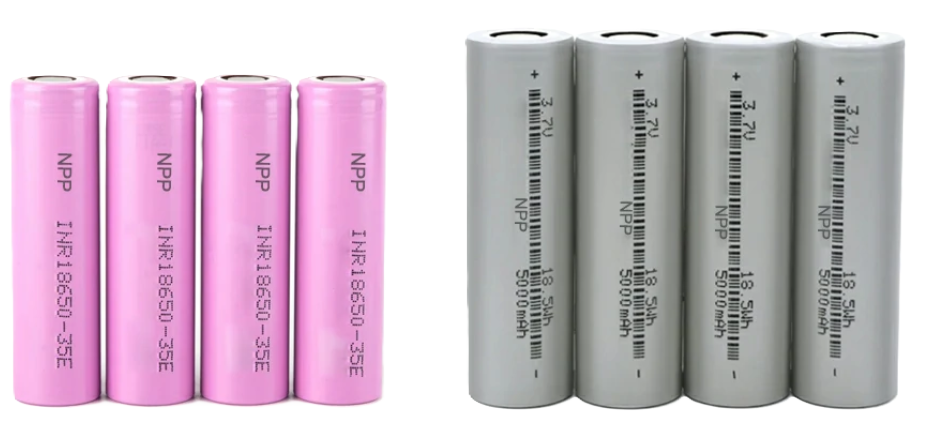 18650 vs 21700 cells
Pouch cells: Pouch cells have a flat and non-standard shape. Unlike cylindrical cells, there is no standard size for pouch cells, and their dimensions can vary widely. As we will discuss later, in general, the larger the cell size, the lower the discharge rate it can support.
Pouch cells are known for their ability to be customized in size and shape, making them suitable for applications where space is a limiting factor, such as in electric vehicles and portable electronics. However, this flexibility in size can sometimes lead to trade-offs in terms of structural stability and discharge performance.
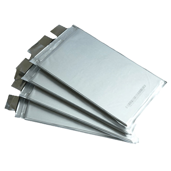 Pouch cells
Discharge Rate
In my opinion, this is the most important characteristic of the battery for our application. As mentioned earlier, the prototype needs to complete 6 laps around the Motorland circuit, with each lap taking approximately 2 minutes and 10 seconds. This translates to:
This means that our battery would need to discharge completely from 100% to 0% within 13 minutes (assuming the worst-case scenario). Not all batteries are capable of handling this fast discharge. Generally, batteries with higher energy density tend to have lower discharge rates, but what exactly is the discharge rate?
The discharge rate, often denoted as “C”, measures the speed at which a battery can discharge relative to its total capacity. Specifically, it refers to the electric discharge current that a battery can deliver based on its total capacity.
For better understanding, let’s use an example:
A cell with a capacity of 4000mAh and a 1C discharge rate means that the battery could provide a maximum of 4000mA (or 4A) over the course of one hour. It could also discharge at 0.5C, meaning it would supply 2000mA (2A) for 2 hours.
If the battery discharged at 2C, it would be able to deliver 8000mA (8A) for 30 minutes, and so on.
| Cs | Discharge rate | Discharge time |
| 0.1 C | 400 mA (0,4A) | 10 hours |
| 0.2C | 800 mA (0,8A) | 5 hours |
| 0.5C | 2000 mA (2A) | 2 hours |
| 1C | 4000 mA (4A) | 1 hour |
| 2C | 8000 mA (8A) | 30 minutes |
| 3C | 12000 mA (12A) | 20 minutes |
| 4C | 16000 mA (16A) | 15 minutes |
| 5C | 20000 mA (20A) | 12 minutes |
| 6C | 24000 mA (24A) | 10 minutes |
| 7C | 28000 mA (28A) | 8,5 minutes |
| 8C | 32000 mA (32A) | 7,5 minutes |
| 9C | 36000 mA (36A) | 6,6 minutes |
| 10C | 40000 mA (40A) | 6 minutes |
It’s important to note that this discharge rate applies equally to our application, regardless of the battery type. Whether we have a 70Ah or a 90Ah battery, if we cannot discharge it completely within those 13 minutes, we will be carrying unnecessary battery weight.
Battery Charging
When it comes to charging batteries, we must consider the following:
Charging methods:
-
Fast charging: The battery charges in significantly less time, which is its primary advantage. However, frequent fast charging can shorten the battery’s lifespan, as it generally increases temperature, among other factors. Additionally, this method often results in a more unbalanced battery, as the Battery Management System (BMS) has insufficient time to balance the cells properly.
-
Slow charging: This method takes considerably longer to charge the battery. On the other side, it’s much healthier for the battery, as it occurs at a lower temperature and allows for cell balancing during the charging process.
Charging strategy:
The charging strategy employed for these batteries is CC-CV (Constant Current - Constant Voltage). Let’s take a closer look at this with an example:
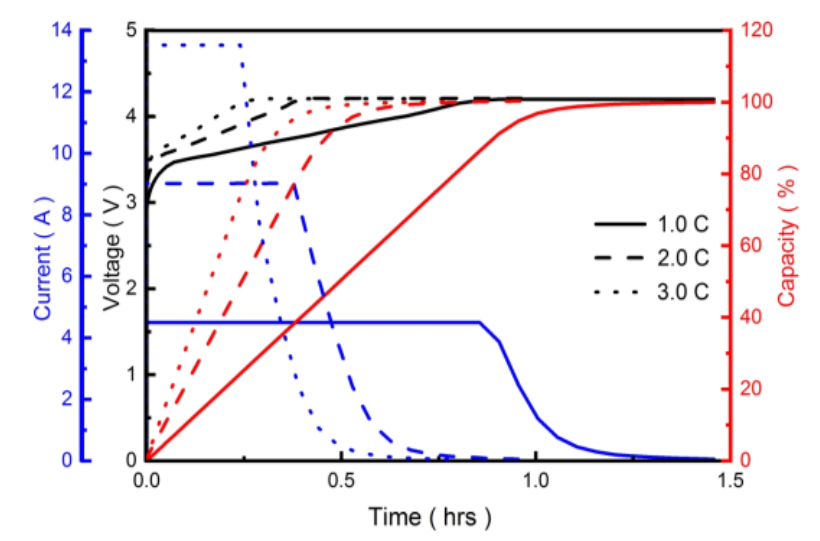 Charging curves
-
CC (Constant Current): This mechanism involves limiting the charging current, typically used during the initial phases of charging when the voltage is low. As illustrated in the charging curve, the blue line remains constant while the voltage (represented by the black line) increases.
-
CV (Constant Voltage): Once the maximum voltage of the battery is reached (it doesn’t mean that is fully charged), we must switch to constant voltage. This means we limit the charging voltage to the maximum level of the battery, allowing the current to decrease gradually until the battery is fully charged.
Another notable characteristic is that approximately 90% of the battery’s charge is achieved during the first 75% of the charging time, while the remaining 10% of the charge takes an additional 25% of the time.
Furthermore, we can consider the charging process complete when the battery’s current consumption drops to just a few milliamperes. Typically, this information can be found in the manufacturer’s datasheet, which may indicate a “cut-off” current, such as 50mA. This means that when the battery’s charging current falls to 50mA or lower, we can assume the battery is fully charged.
In the case of our application, we have over an hour between tests, so the selected cell would be suitable if it can charge at a rate of 1C or more.
Cell Comparation
The first thing we need to do is to perform an evaluation of the cells available in the market. After doing a lot of research, we analyzed the following cells:
| Cell | Format | Capacity | Continuous discharge | Maximum discharge | Density (wh/L) |
| Samsung 15Q | 18650 | 1.5 Ah | 18A (12C) | - | 317 Wh/L |
| Sanyo RX | 18650 | 2.05Ah | 20A (9C) | - | 412 Wh/L |
| LG Chem HD2 | 18650 | 2.0 Ah | 20A (10C) | - | 438 Wh/L |
| Sony VTC6 | 18650 | 3.0 Ah | 15A (5C) | 30A (10C) - 80ºC | 634 Wh/L |
| Sony VTC5 | 18650 | 2.6 Ah | 10A (4C) | 20A (8C) | 570 Wh/L |
| Sony VTC5A | 18650 | 2.6 Ah | - | 35 A (13C) - 80ºC | 528 Wh/L |
| Sony VTC4 | 18650 | 2.1 Ah | 20 A (10C) | 30A (7C) | 474 Wh/L |
| TerraE 32P | 18650 | 3.1 Ah | 20A (6C) | 30A (10C) - 80ºC | 655 Wh/L |
| Samsung 22P | 18650 | 2.1 Ah | 10 A (5C) | - | 450 Wh/L |
| Molicel P26A | 18650 | 2.6 Ah | 20 A (8C) | 35 A (13C) | 559 Wh/L |
| LG HE4 | 18650 | 2.5 Ah | 20 A (8C) | - | 514 Wh/L |
| Acebeam 25A | 18650 | 3.1 Ah | 20 A (6C) | 25 A (8C) | - |
| Samsung 25R | 18650 | 2.5 Ah | 20 A (8C) | 30A (12C) | - |
| Molicel P28A | 18650 | 2.8 Ah | 30A (11C) | 35 A (13C) | 569 Wh/L |
| LG Chem M29 | 18650 | 2.85 Ah | 6 A (2C) | 10 A (4C) | 603 Wh/L |
| BAK Battery CL-29 | 18650 | 2.9 Ah | 6.5 A (2C) | 12.5 A (4C) | 627 Wh/L |
| DMEGC 29E | 18650 | 2.85 Ah | 10 A (4C) | 15 A (5C) | - |
| Samsung 30Q | 18650 | 3.0 Ah | 15 A (5C) | - | 645 Wh/L |
| Samsung 30T | 21700 | 3.0 Ah | 35 A (12C) | - | 468 Wh/L |
| Samsung 40T | 21700 | 4.0 Ah | 35 A (9C) | 45 A (11C) - 80ºC | 573 Wh/L |
| Molicel P42A | 21700 | 4.2 Ah | 45 A (10C) | - | 570 Wh/L |
| Molicel P45B | 21700 | 4.5 Ah | 40 A (9C) | 45 A (10C) - 80ºC | 668 Wh/L |
| Samsung 50s | 21700 | 5.0 Ah | 25 A (5C) | 45 A (9C) - 80 ºC | 742 Wh/L |
| LG M58T | 21700 | 5.5 Ah | 12.5 A (2C) | 15 A (3C) | 796 Wh/L |
| LG Chem E66A | Pouch | 65 Ah | 121 A (2C) | 297 A (5C) | 500 Wh/L |
| LG Chem F2 | Pouch | 6.5 Ah | 130 A (20C) | 256 A (40C) | 171 Wh/L |
| LG Chem E63B | Pouch | 63 Ah | 63 A (1C) | 189 A (3C) | 598 Wh/L |
| Kokam KCL216057PN1 | Pouch | 57 Ah | 456 A (8C) | 570(10C) | 459 Wh/L |
| Kokam KCL355087PS0 | Pouch | 87 Ah | 783 A (9C) | 1044(12C) | 462 Wh/L |
| Grepow A942126 | Pouch | 7.6 Ah | 90 A (11C) | - | 495 Wh/L |
| Grepow 8265146 | Pouch | 9.7 Ah | 97 A (10C) | - | 484 Wh/L |
Regarding the table above, it’s important to note that our primary interest lies in the continuous discharge column. It’s essential to comment that there is no standard by which manufacturers indicate the maximum discharge rate. Some report the discharge until the cell reaches 80°C and stop the test, while others provide the rate based on time pulses, meaning the duration the cell can deliver that intensity in a peak form.
On the other hand, the cells marked in orange are those that could initially be valid but have been discarded for the following reasons:
- TerraE 32P: This cell comes from a less-known brand and doesn’t offer any advantages compared to the other selected 18650 cells.
- Acebeam 25A: This cell has a very high price considering the characteristics it offers compared to others. Additionally, its positive terminal is not designed for soldering, which is another reason for its exclusion.
- Samsung 50S: Although it theoretically supports a 5C discharge rate, numerous reports indicate that the cell reaches temperatures of 90°C when discharging at that current.
- Kokam: The manufacturer does not sell directly to individuals or in small quantities, they require a minimum purchase of 200 cells and we only new a few as they are big cells.
- Grepow: The delivery times were excessively long for our deadlines.
LiPo Cells
After researching different brands, we contacted Melasta and Grepow, Chinese manufacturers of LiPo cells, and obtained information about the cells they manufacture. In this case, we were able to analyze 160 cells.
From our analysis, we observed the following:
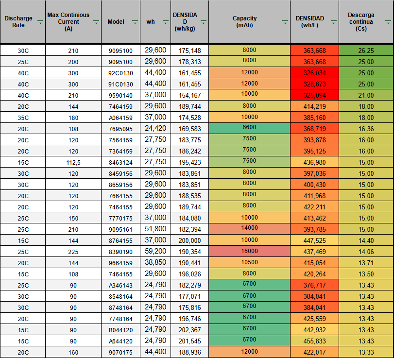 LiPo cell data12
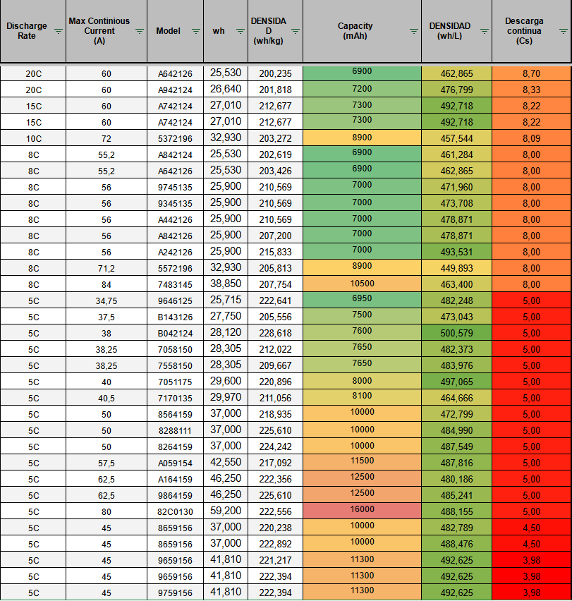 LiPo cell data12
As we can see, these batteries provide a commendable discharge rate for our application. The colored map columns illustrate the cell capacity, energy density, and allowable discharge rate.
It’s evident that as the energy density of a cell increases, its discharge rate tends to decrease. This aligns with the data we can obtain from two very similar cylindrical cells, the Samsung 40T and Samsung 50S. Although both are the same size, the Samsung 50S has a higher energy density but a lower discharge rate.
Furthermore, we can observe that, generally, larger cell sizes correlate with lower discharge rates. In cases where a larger cell accommodates a high discharge rate, its energy density will typically be lower.
Unfortunately, the pricing for these cells was significantly higher, approximately three times the cost of cylindrical cells under the same conditions, and the delivery timelines were too lengthy to meet our deadlines. As a result, we didn’t pursue this type of battery and were unable to conduct tests on these models to verify the provided specifications.
Cell Testing
After analyzing the cells that could meet our specifications, we proceeded to purchase samples of the models that seemed most promising. Additionally, we conducted tests with other models that we had available.
Different types of cells tested
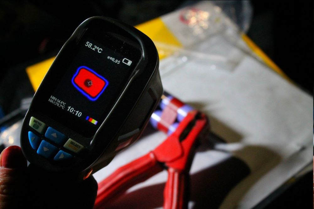 Cell temperature measurement
The tested cells, as shown in the image, were:
- Brutepower 22,000 mAh (NXE Power)
- Tattu 22,000 mAh 30C 6S
- Sony VTC6
- Molicel P28A
- Samsung 30Q
- Molicel P42A
- Molicel P45B
- Samsung 40T
- LG Chem E63B
Our main objectives were to determine whether they provided the capacity indicated by the manufacturer, if they could support the discharge current we needed, and the maximum temperature of each cell.
During the tests, we measured the actual capacity of the batteries, the maximum discharge current, and the maximum temperature reached. For this purpose, we used a battery discharger like the one shown below:
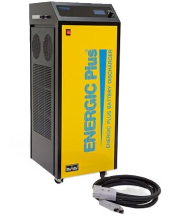 Discharger
The operation of this type of discharger essentially involves dissipating electrical energy as heat through resistors and fans. It’s important to note that this discharger was designed for batteries around 100V and allows for discharges of up to 200A. Due to its internal functioning, when discharging cells at approximately 3.7V, the discharge current decreases as the voltage drops. I suspect it has different internal stages, and we were only using one at that voltage.
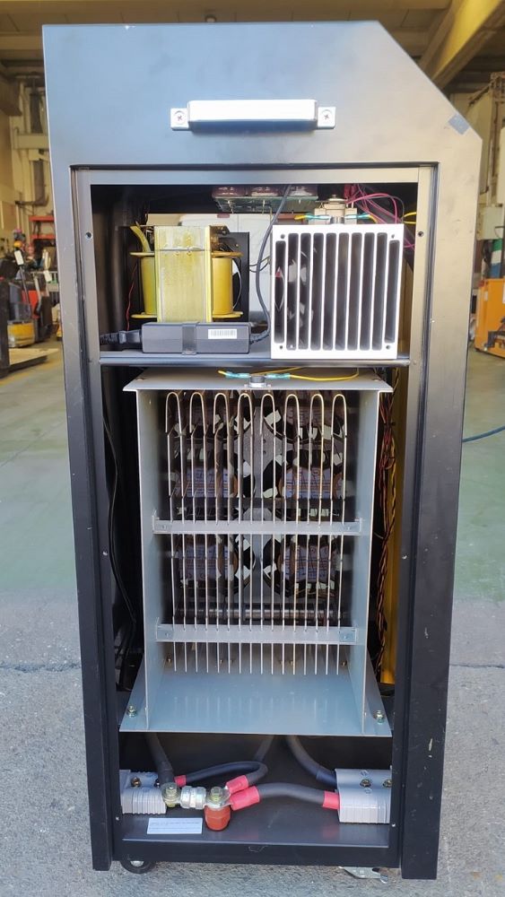 Left view |
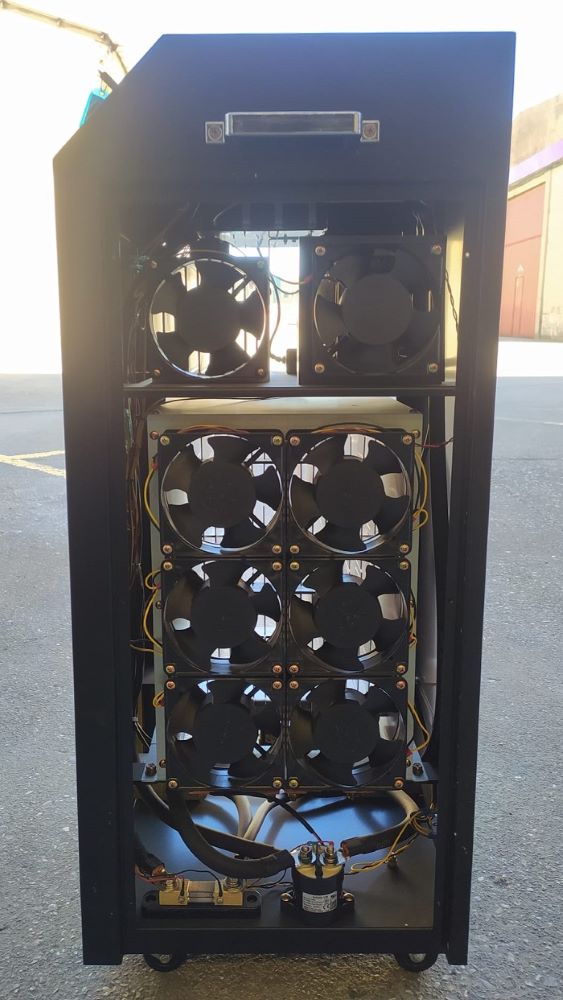 Right view |
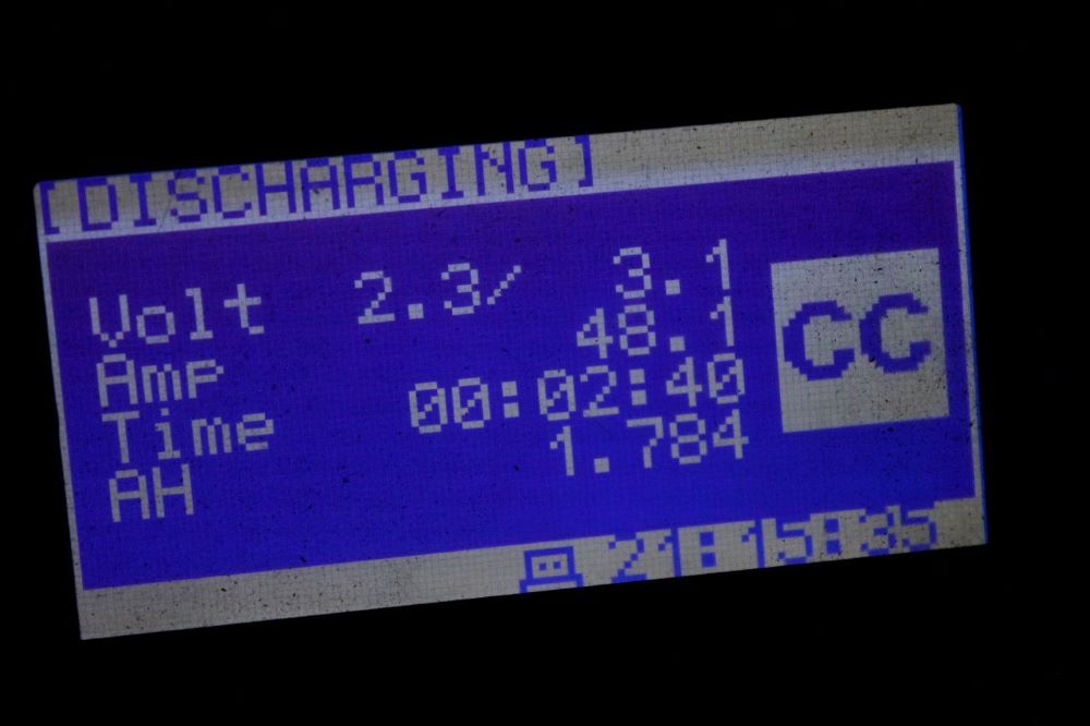 Discharger display
Test Environment
The ideal test would have involved generating a variable discharge pattern based on telemetry from the circuit to simulate the most realistic scenario possible. It’s important to note that during the competition, we don’t experience continuous discharge but rather discharge peaks that correspond to the inverter’s consumption. Additionally, these peaks will exceed the discharge intensity that we could simulate at the necessary C rates. Due to time constraints and the resources available, this test was performed under continuous discharge conditions only.
The tests were also conducted during winter, with ambient temperatures between 10°C and 15°C. While I recognize this is not an ideal testing environment, we were pressed for time and needed to make a decision quickly.
It’s worth noting that some discharges went down to 2.3V because the discharger has a voltage reading error of 0.2V, which was accounted for by setting the cutoff to 2.3V.
Note: The tests were conducted at different voltages, and current consumption decreased as voltage dropped. This is due to the discharger’s design, which operates optimally at around 100V, allowing for a discharge of 200A. However, at lower voltages, it couldn’t discharge the requested current (likely due to its internal construction). In the second test, to reach 120A, we used two cells in series. This had no impact on the results, and the tests can be considered equivalent.
Below are the results of the tests conducted.
Brutepower 22000 mAh 6s (NXE Power)13
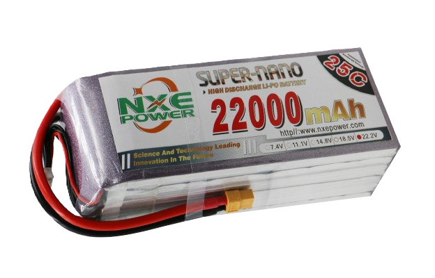 NXE Power
| Feature | Value |
| Brand | NXE Power |
| Model | 12090193SH25 |
| Format | Pouch |
| Chemistry | LiPo |
| Maximum voltage | 4.2V |
| Nominal voltage | 3.7V |
| Minimum voltage | 3V |
| Capacity | 22000 mAh (22Ah) |
| Peak discharge | 550A (25C) |
| Maximum continuous dicharge | 22A (1C) |
| Continuous charging | 22A (1C) |
| Maximum charging | 44A (2C) |
| Maximum temperature | 60ºC |
| Weight | 440g |
We have a battery built with 6 cells in series, which limits our flexibility during the manufacturing process. However, having this series configuration doesn’t affect our tests. These cells were used by the team in the previous edition of the competition. Brutepower is a rebranding, and if I remember correctly, NXE Power was the original manufacturer.
Tests
Test 1: 50A (2.5 C) discharge
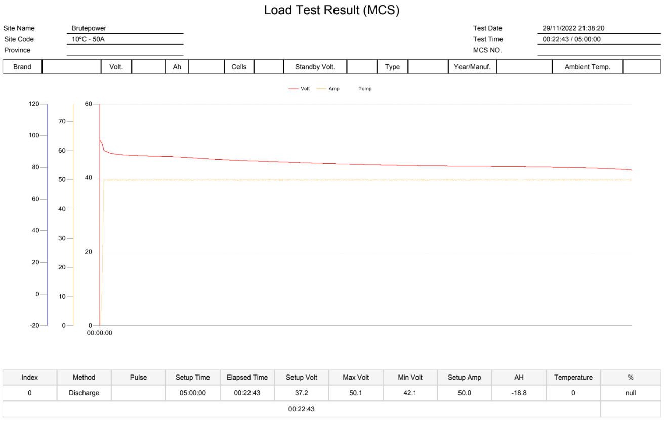 50A (2.5C) discharge
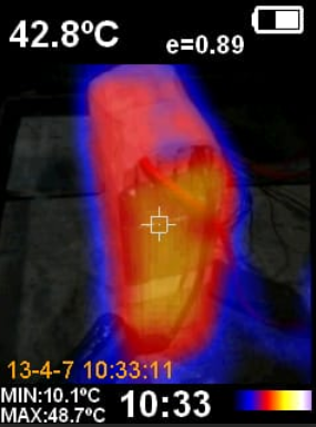 Final temperature
Test 1 results
| Property | Value |
| Initial temperature | 10 ºC |
| Final temperature | 43 ºC |
| Initial voltage | 4.2V (12 cells) |
| Final voltage | 3.5V (12 cells) |
| Discharge rate | 50A (2.5C) |
| Measured capacity | 18,8 Ah |
| Test time | 22 minutes |
In this test, we stopped the discharge due to the high temperature reached by the cell, which was 43ºC on its outer surface. Although the theoretical maximum temperature is 60ºC, we wanted to avoid damaging the battery or pushing it to its limits. Despite this, the cell was still far from the 5C discharge rate we were aiming for.
Test 2: 44A (2C) discharge
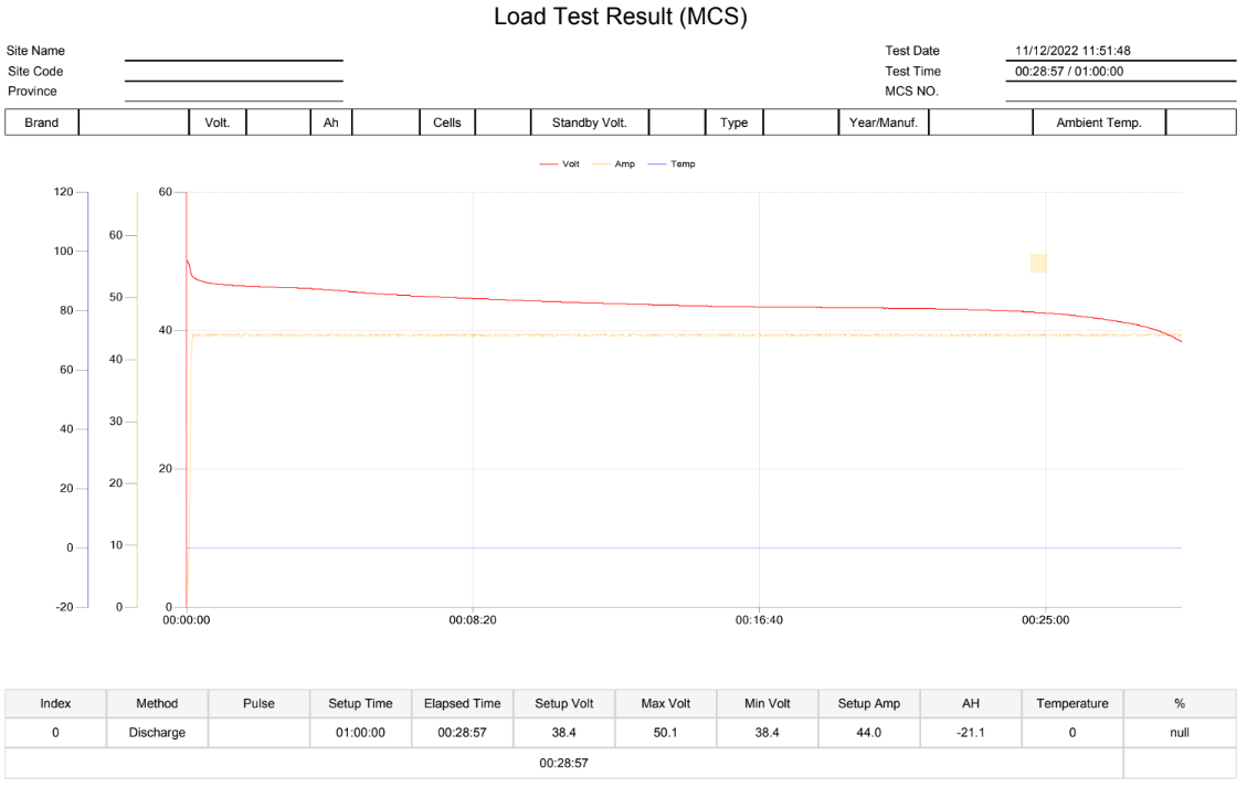 44A (2C) discharge
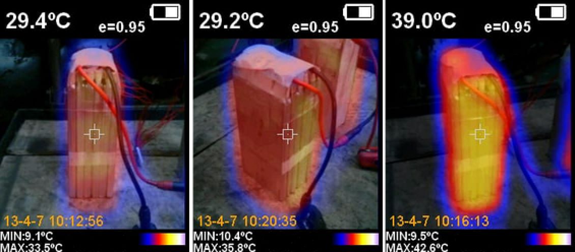 Final temperature
Test 2 results
| Property | Value |
| Initial temperature | 10 ºC |
| Final temperature | 39 ºC |
| Initial voltage | 4.2V |
| Final voltage | 3.2V |
| Discharge rate | 44A (2C) |
| Measured capacity | 21,1 Ah |
| Test time | 28 minutes |
Summary
As seen in these tests, the cells are capable of delivering a maximum discharge rate of around 2C, which makes them unsuitable for our application. Moreover, the data from the Melasta manufacturer confirms that a 22Ah cell like this cannot sustain a discharge rate higher than 2C.
Remember when I mentioned at the beginning of this article that the previous team chose these batteries for the prototype? This is the reason why they are not valid for this application.
Invalid
LG Chem E63B141516
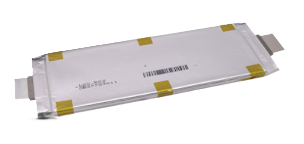 LG Chem E63B cell
| Feature | Value |
| Brand | LG |
| Model | E63B |
| Format | Pouch |
| Chemistry | NMC |
| Maximum voltage | 4.2V |
| Nominal voltage | 3.6V |
| Minimum voltage | 2.5V |
| Capacity | 63000 mAh (63 Ah) |
| Peak discharge | 189A (3C) |
| Maximum continuous discharge | 63A (1C) |
| Charge rate | 18.9A |
| Maximum charge rate | 31A (0.5C) |
| Maximum temperature | 60 ºC |
| Weight | 882g |
Tests
Test 1: 60A (1C) discharge
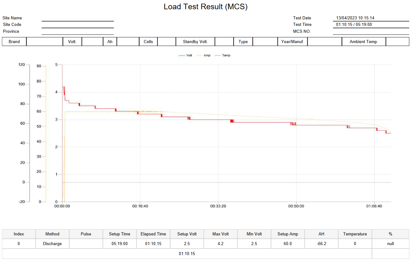 60A (1C) discharge
Test 1 results
| Property | Value |
| Initial temperature | 15ºC |
| Final temperature | 35 ºC |
| Initial voltage | 4.2 V |
| Final voltage | 2.5 V |
| Discharge rate | 60A (1C) |
| Measured capacity | 66,2 Ah |
| Test time | 1 hour 10 minutes |
Test 2: 120A (2C) discharge
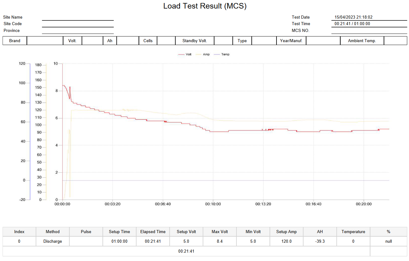 120A (2C) discharge
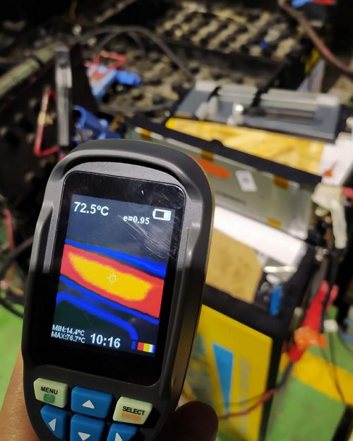 Final external temperature |
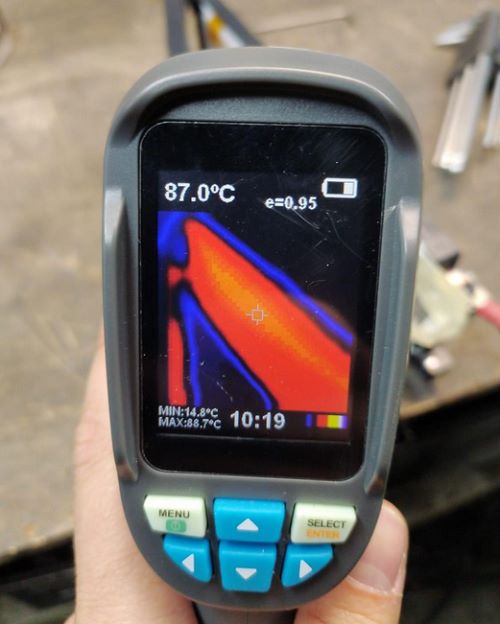 Final internal temperature |
Test 2 results
| Property | Value |
| Initial temperature | 15 ºC |
| Final temperature | 87 ºC (Stopped because of high temperature) |
| Initial voltage | 4.2 V |
| Final voltage | 2.5V (Stopped because of high temperature) |
| Discharge rate | 120A (2C) |
| Measured capacity | 39,3 Ah (Stopped because of high temperature) |
| Test time | 21 minutes (Stopped because of high temperature) |
Summary
This cells have a good density, they are cheap and almost using one module would be enough for the capacity we are looking for. However, they have two problems, the first one is the modularity. We could not install for example 90Ah, only 60Ah or 120Ah (2 cells in parallel). But the main reason is that in the test carried out previously, these cells don’t even allow a 2C discharge, so it’s far from the 4C-5C that we are looking for. As a curiosity, you can see in the second test how the voltage has a rather strange behavior on the graph, especially at the end of the graph. This instability is probably due high temperature.
Invalid
Sony VTC617
 Sony VTC6 cells
| Feature | Value |
| Brand | Sony |
| Model | US18650VTC6 |
| Format | 18650 |
| Maximum voltage | 4.25V |
| Nominal voltage | 3.6V |
| Minimum voltage | 2.0V |
| Capacity | 3000 mAh (3Ah) |
| Peak discharge | 30A (10C) |
| Maximum discharge rate | 15A (5C) |
| Charging rate | 5A (1.6C) |
| Maximum charging rate | 6A (2C) |
| Maximum temperature | 80 ºC |
| Weight | 46.6g |
Tests
Test 1: 15A (5C) discharge (3 parallel cells)
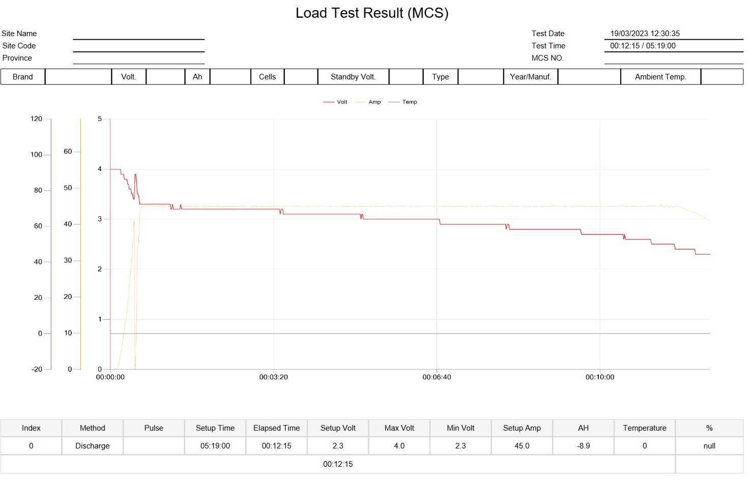 15A (5C) discharge
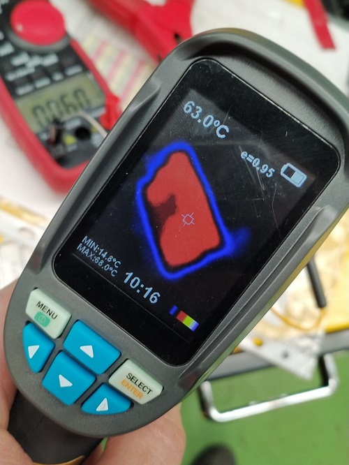 Final temperature
Test 1 results
| Property | Value |
| Initial temperature | 15 ºC |
| Final temperature | 63 ºC |
| Initial voltage | 4.2 V |
| Final voltage | 2.5V |
| Discharge rate | 15A (5C) |
| Measured capacity | 3 Ah (3 cells in parallel) |
| Discharge time | 12 minutes |
Summary
The first thing to mention is that the test was performed with 3 cells in parallel. Of course, when performing this type of tests, the currents are scaled to maintain the discharge at 5C. In this case, having 3 cells of 3Ah each (9Ah) we discharge at 5C on those 9Ah, that is to say at 45A of discharge. We found these cells valid for our application. Perhaps, the only disadvantage is the size and the large number of them that we would have to install, but they are perfectly valid.
Valid
Molicel P28A18
 Molicel P28A
| Feature | Value |
| Brand | Molicel |
| Model | INR-18650-P28A |
| Format | 18650 |
| Maximum voltage | 4.2V |
| Nominal voltage | 3.6V |
| Minimum voltage | 2.5V |
| Capacity | 2800 mAh (2.8Ah) |
| Peak discharge | 35A (12.5C) |
| Maximum discharge rate | 20A (7C) |
| Charging rate | 2.8A (1C) |
| Maximum charging rate | 6A (2.1C) |
| Maximum temperature | 60ºC |
| Weight | 46g |
Tests
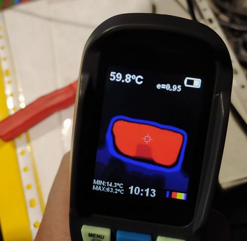 Final temperature
Summary
Unfortunately, I lost the discharge graph of this cell, but this cell met the specifications for our application. The negative point is the cell format that is small and we need too many cells.
Valid
Samsung 30Q19
 Samsung 30Q
| Feature | Value |
| Brand | Samsung |
| Model | INR18650-30Q |
| Format | 18650 |
| Chemistry | NCA |
| Maximum voltage | 4.2V |
| Nominal voltage | 3.6V |
| Minimum voltage | 2.5V |
| Capacity | 3000 mAh (3Ah) |
| Peak discharge | 20A (6C) |
| Maximum discharge rate | 15A (5C) |
| Charging rate | 1.5A (0.5C) |
| Maximum charging rate | 4A (1.3C) |
| Maximum temperature | 75 ºC |
| Weight | 45.6 g |
Tests
Test 1: 15A (5C) discharge (3 parallel cells)
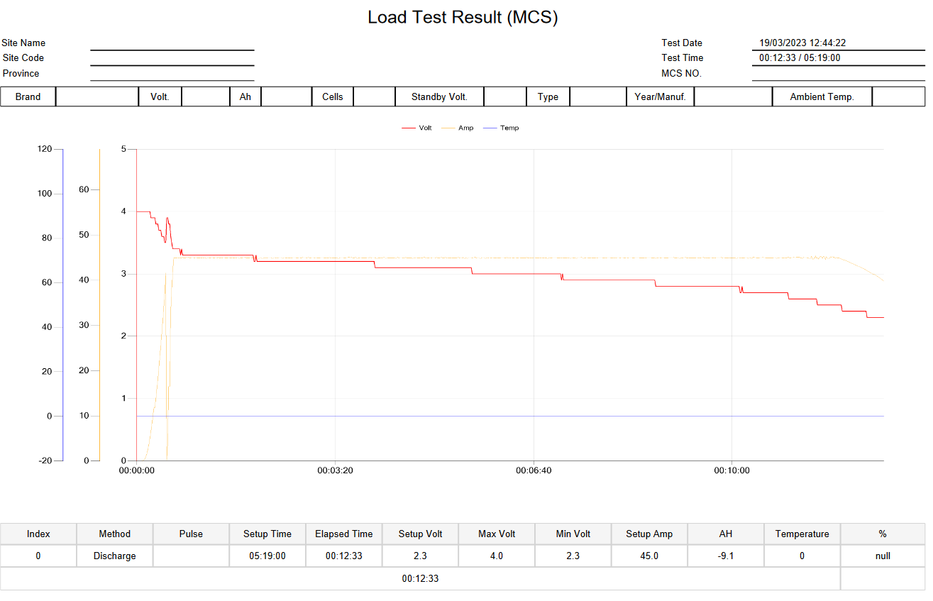 15A (5C) discharge
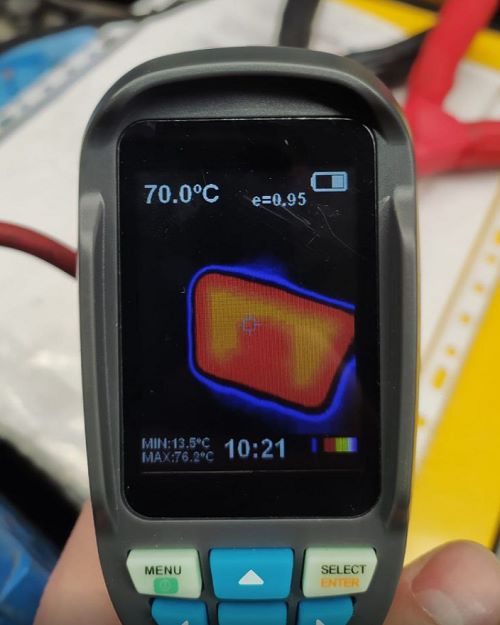 Final temperature
Test 1 results
| Property | Value |
| Initial temperature | 15 ºC |
| Final temperature | 70 ºC |
| Initial voltage | 4.2 V |
| Final voltage | 2.5V |
| Discharge rate | 15A (5C) |
| Measured capacity | 3 Ah (3 parallel cells) |
| Discharge time | 12 minutes |
Summary
As before, the test was performed with 3 cells in parallel, so to get the 5C we discharged at 45A. In the graph we can see how at a certain moment the current drops, this is due to the operation of the discharger and the work stages, as we mentioned before.
In this case we can find these cells as valid for our application although it is true that they have a fairly high temperature, but within the specification.
Valid
Molicel P42A20
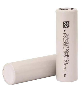 Molicel P42A
| Feature | Value |
| Brand | Molicel |
| Model | INR-21700-P42A |
| Format | 21700 |
| Maximum voltage | 4.2V |
| Nominal voltage | 3.6V |
| Minimum voltage | 2.5V |
| Capacity | 4200 mAh (4.2Ah) |
| Peak discharge | - |
| Maximum discharge rate | 45A (10C) |
| Discharge rate | 4.2A (1C) |
| Maximum charge rate | - |
| Maximum temperature | 60 ºC |
| Weight | 70g |
Tests
Test 1: 21A (5C) discharge (2 parallel cells)
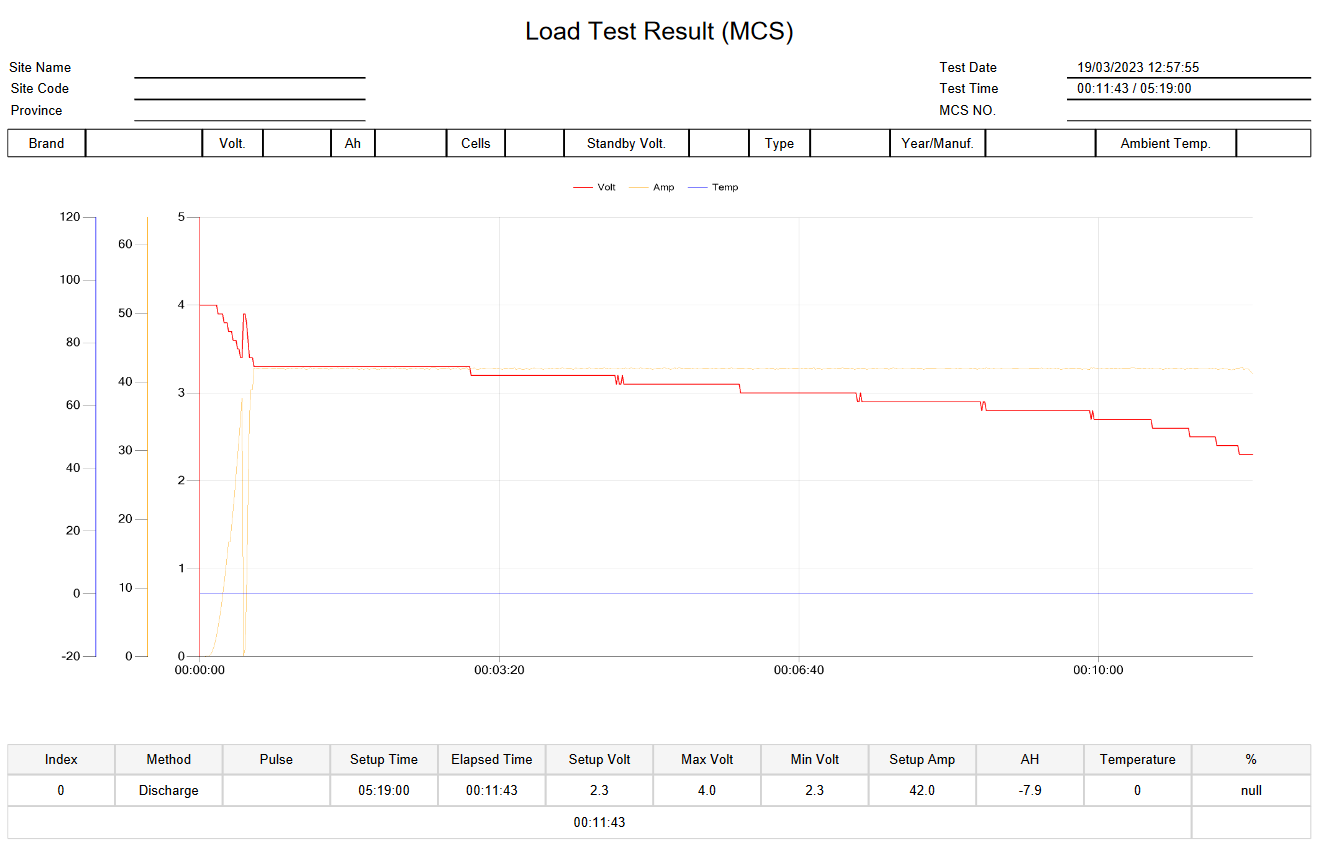 21A (5C) discharge
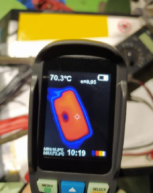 Final temperature
Test 1 results
| Property | Value |
| Initial temperature | 15 ºC |
| Final temperature | 70 ºC |
| Initial voltage | 4.2 V |
| Final voltage | 2.5V |
| Discharge rate | 21A (5C) |
| Measured capacity | 4 Ah (2 parallel cells) |
| Discharge time | 11 minutes |
Summary
As we can see on the test, the discharge has been done with 2 cells in parallel. Perhaps this model is the one that compared with similar other cells, has given us the worst results with a high temperature of 70 ºC and 0.2Ah less capacity than the advertised one. Even so, it’s valid for our application.
Valid
Samsung 40T21
 Samsung 40T
| Features | Value |
| Brand | Samsung |
| Model | INR21700-40T |
| Format | 21700 |
| Maximum voltage | 4.2V |
| Nominal voltage | 3.6V |
| Minimum voltage | 2.5V |
| Capacity | 4000 mAh (4 Ah) |
| Peak discharge | 45A (11C) |
| Maximum discharge rate | 35A (8C) |
| Charge rate | 2A (0.5C) |
| Maximum charge rate | 6A (1.5C) |
| Maximum temperature | 80 ºC |
| Weight | 70g |
Tests
Test 1: 20A (5C) discharge (3 parallel cells)
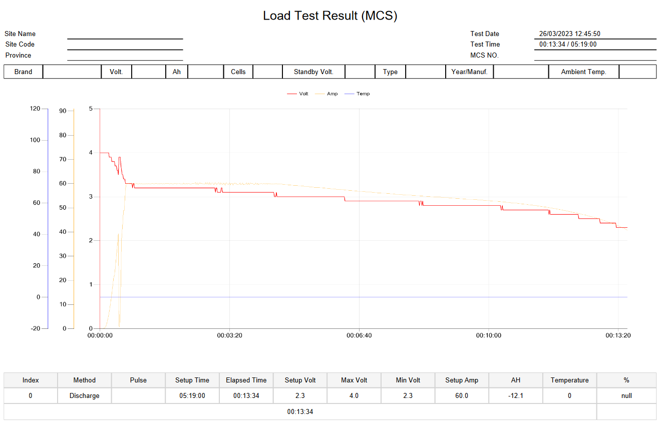 20A (5C) discharge
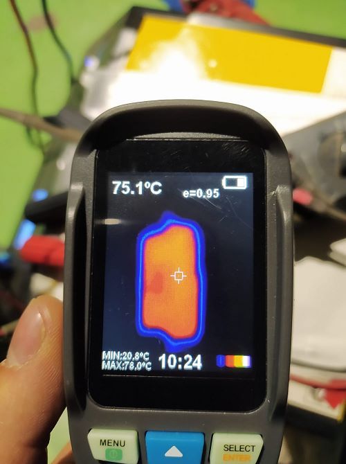 Final temperature
Test 1 results
| Property | Value |
| Initial temperature | 17 ºC |
| Final temperature | 75 ºC |
| Initial voltage | 4.2 V |
| Final voltage | 2.5V |
| Discharge rate | 20A (5C) |
| Measured capacity | 4 Ah (3 parallel cells) |
| Discharge time | 13 minutes |
Summary
The cells have met the specifications and although they reached high temperature (75ºC), it’s within the 80ºC range set by the manufacturer so they are perfectly valid.
Valid
Molicel P45B22
 Molicel P45B
| Feature | Value |
| Brand | Molicel |
| Model | INR-21700-P45B |
| Format | 21700 |
| Maximum voltage | 4.2V |
| Nominal voltage | 3.6V |
| Minimum voltage | 2.5V |
| Capacity | 4500 mAh (4.5Ah) |
| Peak discharge | - |
| Maximum discharge rate | 45A (10C) Cutting at 80ºC |
| Charge rate | 4.5A (1C) |
| Maximum charge rate | 13A (2.8C) Cutting at 70ºC |
| Maximum temperature | 80 ºC |
| Weight | 70g |
Tests
Test 1: 22.5A (5C) discharge (3 parallel cells)
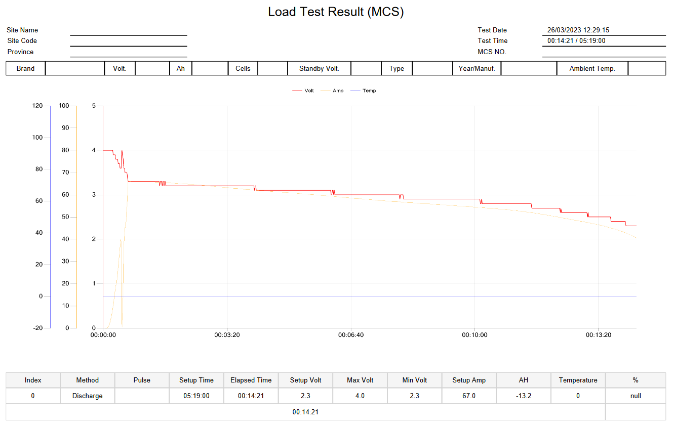 22.5A (5C) discharge
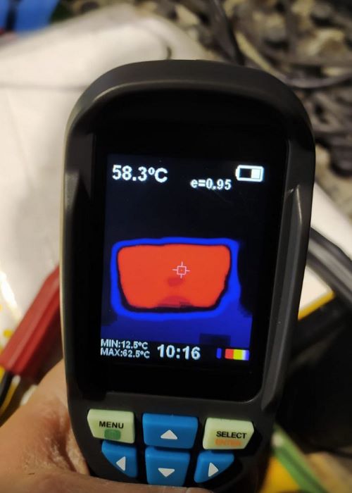 Final temperature
Test 1 results
| Property | Value |
| Initial temperature | 12 ºC |
| Final temperature | 58 ºC |
| Initial voltage | 4.2 V |
| Final voltage | 2.5V |
| Discharge rate | 22.5A (5C) |
| Measured capacity | 4.4 Ah (3 parallel cells) |
| Discharge time | 14 minutes |
Summary
As we can see these cells also meet the specifications. From my point of view they could be considered the best because they reach lower temperature than the other tested cells of this size and they are the ones with the highest energy density.
Performing a discharge test at 6C the cells reached a temperature of 67ºC with an ambient and initial temperature of 15ºC.
Valid
Final Decision
The tests completed previously give us an idea of which cells are valid or not. Nonetheless, we conducted several additional tests to continue removing options and reach a final decision. Below is a summary of the average results obtained:
| Cell | Format | Datasheet capacity | Measured capacity | Final temperature |
| Sony VTC6 | 18650 | 3.0 Ah | 3.0 Ah | 63.0 ºC |
| Molicel P28A | 18650 | 2.8 Ah | 2.7 Ah | 60.0 ºC |
| Samsung 30Q | 18650 | 3.0 Ah | 3.0 Ah | 70.0 ºC |
| Molicel P42A | 21700 | 4.2 Ah | 4.0 Ah | 70.0 ºC |
| Samsung 40T | 21700 | 4.0 Ah | 4.0 Ah | 75.0 ºC |
| Molicel P45B | 21700 | 4.5 Ah | 4.4 Ah | 60.0 ºC |
The best cell was Molicel P45B, so we decided to use it for our battery.
Electrical Structure of the Battery
Talking about the electrical structure of the battery, we have 3 designs for its manufacture:
1. Series-parallel configuration: This means making the connections first in series and then in parallel as we can see in the diagram below:
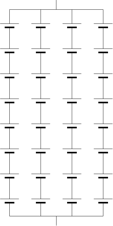 Series-parallel configuration
-
Advantages: With this configuration we reduce the use of conductive materials during manufacturing since the total current of the battery is concentrated in each of the terminals.
-
Disadvantages: High complexity in monitoring and charging. With this configuration we would need to have balancing wires in absolutely all the cells, as well as a BMS for each parallel line that we add.
Obviously the advantage that it gives us is much less than the disadvantage, so we discard this system.
2. Parallel-series configuration: This configuration consists of making the connections in parallel and then in series.
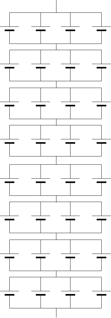 Parallel-series configuration
-
Advantages: Simple manufacturing and control. With a single BMS we are able to control the entire battery.
-
Disadvantages: The current flows through all the series so we need a greater amount of conductor to support the current.
3. Mixed configuration: In this configuration both systems are mixed. For example we can have a battery built by series-parallel-series. An example would be if we had a battery with 6s modules that we could not separate. We would have to do series and parallel again to get the battery we need.
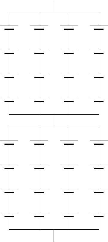 Series-parallel-series configuration
This configuration is appropriate if we only have this option by buying batteries that have the series made and we cannot separate them easily.
It has the advantages and disadvantages of the previous configurations at an intermediate point. The balancing system is more complex than in the second case but simpler than in the first. Likewise, the circulation of the current is better than in the second case but worse than in the first.
After deciding between the second and third options, we decided on the second option, that is, a parallel-series battery.
Mechanical Structure of the Battery
Introduction
Once we selected the cells we were going to use and understood their capacity and characteristics, we began working on the battery design. The first step was to determine the configuration we would use. We knew we needed 28 cells in series to get as close as possible to the 120V limit imposed by the inverter. The decision that remained was the number of cells to use in parallel.
Based on some data we found online about the circuit and attempting to estimate the consumption of the electric motor (as we hadn’t made much progress on the power bench yet and needed to make a decision), we established 20 cells in parallel.
Unfortunately, our calculations were incorrect for two main reasons:
Incorrect consumption estimation: Since we hadn’t advanced much with dyno, we relied on the consumption and power ratings indicated on paper for the motor. The issue was that this information was overstated. In reality, the motor was not able of delivering as much power as indicated. We were not the only team to overestimate the battery size.
Inefficiency of motor cooling: As we will see later, these motors can operate at peak power for a few seconds and at nominal values for the rest of the time. We had data on the motor’s consumption from the previous edition, which was air-cooled, and we assumed that this water-cooled motor would dissipate heat better. However, that was not true for this motor.
These two factors, along with a safety margin we added to the battery, caused us to exceed the size we actually needed.
However, at this point, we were clear that the battery would be configured as 28s20p, allowing us to start working on the design.
Cell Structure
One of the requirements we wanted for the battery was to be modular, so that in the event of a failure in one of the modules, we could replace it with a new one without compromising the entire battery. Additionally, since I didn’t have much experience with this type of battery, we decided to design it to allow air flow between the cells. We can arrange the cells mainly in two designs:
- Honeycomb structure: This arrangement of the cells allows for greater density, as it eliminates space between the cells. However, this structure results in worse air circulation between cells.
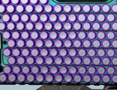 Example of honeycomb structure
- Aligned structure: This configuration was the one we selected because it allowed us to create a square structure, provided sufficient separation between cells, and was straightforward to manufacture.
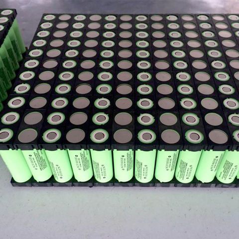 Example of aligned structure
In the market, there are numerous spacers available for battery assembly, but in our case, we needed to create a modular structure, which meant that none of the commercial spacers were suitable.
Battery Design
As mentioned before, we wanted a repairable battery. This means that if one of the cells breaks, we could replace it with a new one and not ruin the whole battery. Of course, doing that is not easy since the cells are welded together, so we had to find a middle point. The battery was going to be a 28s 20p so we decided to sacrifice absolute modularity for less complexity. To do this we created 20p modules which could not be easily disassembled, but the 28s could, so if a cell broke, we had to replace 20 cells and not 560 which were the total of the battery. Also during the design we were focusing on using the least amount of copper as it’s expensive and heavy. With this goals, we started with the battery design.
We tried multiple designs until reach the final one:
Model 1
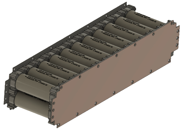 Model 1 module |
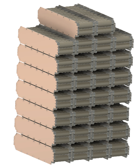 Model 1 complete battery |
Model 2
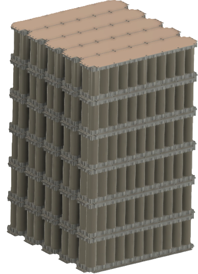 Model 2
Model 3
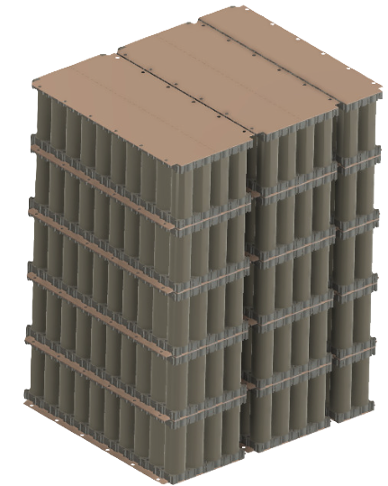 Model 3
Model 4
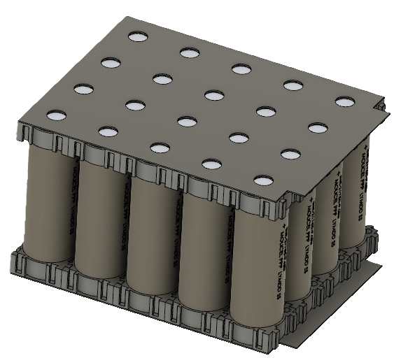 Module of model 4 |
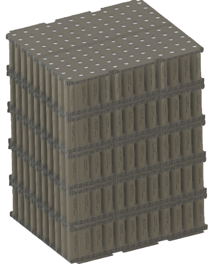 Model 4 |
Model 5
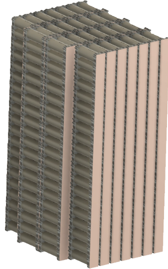 Model 5
Model 6
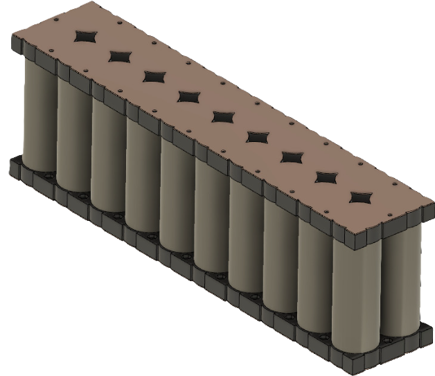 Module of model 6 |
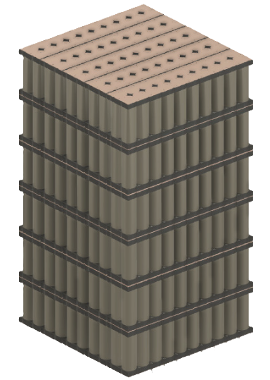 Model 6 |
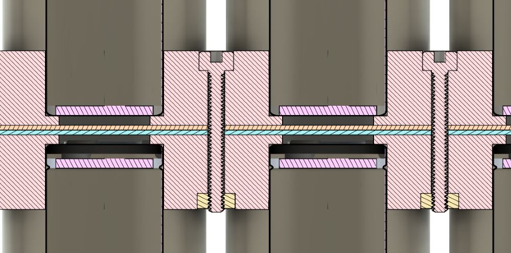 Model 6: Section view of the connections
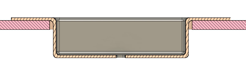 Nickel tab section view
The last design (Model 6) had 3 main problems:
- Assembly complexity: Because there are screws between the cells, the assembly becomes more complex.
- The connection between the copper busbars was not secured: It is not possible due to the design to mount screws on the inside of the module so we can only secure the connection in the outer areas of the battery.
- Nickel tabs: In the manufacture of the busbars, the nickel tabs protrude 0.15 mm above the busbar, so the copper will not be completely in contact, making the connections only by the nickel tabs, which is insufficient.
Final Design
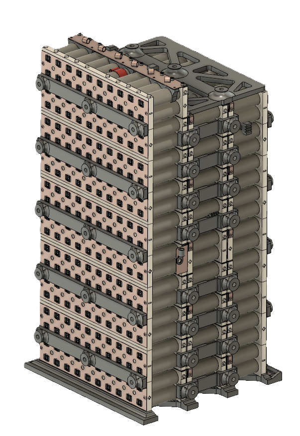 Battery render
As mentioned before, the design is made with 28 modules, each one with 20 cells. At the bottom we have a 3D printed base with PA ensuring a firm surface and a safe insulation with the battery container. The negative terminal is attached with bolts since the cables will be soldered with tin. In this case we have 6 cables which will be joined outside of the container with a busbar that goes to the inverter.
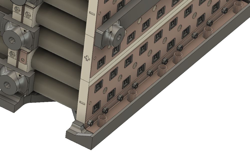 Negative terminal. The power cables will be soldered to the final copper plate with tin and then screwed to the modules to avoid heating the battery cells during the process
On the sides we have spacers held by the screw heads. These spacers will have inserts so once the battery pack is closed, they will be held in place with screws from the outside as well as those found in the front and rear areas.
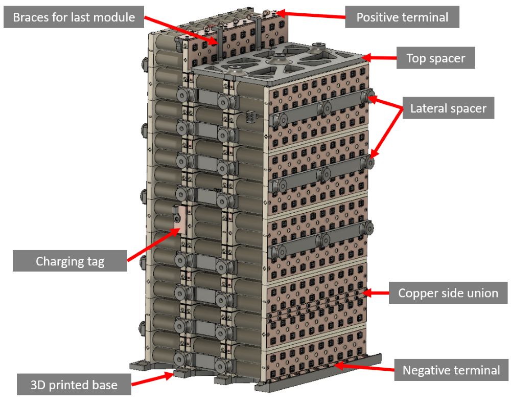
Finally, at the top of the battery we have a spacer that will compress the battery pack when we mount the top cover, securing the complete assembly vertically. since the last module is only held in place by the external connections, two braces have been added to hold it in place. Also, all the 3D printed parts have the right tolerances so everything fits a little tightly and without any slack.
There are two types of copper connections, the lateral ones and the central ones. The central have a tab to be able to mount a terminal and make the connection to the BMS balancing wires.
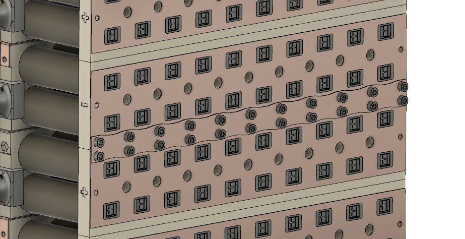 Side connections between modules
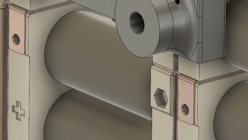 Tabs for BMS balancing wires
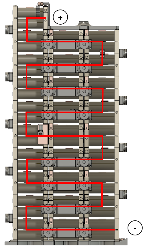 Connection scheme of the series
Another feature is the interchangeability of the 3D printed structure. Between the printed parts, both for guarding and for holding they have square protrusions. These have been designed so that they can be mounted on any of the modules and not have to manufacture different pieces for each one. There are only 3 types of modules, the left, the right and the central one. The red piece is a clamp to hold the temperature sensor of each module, also printed in 3D.
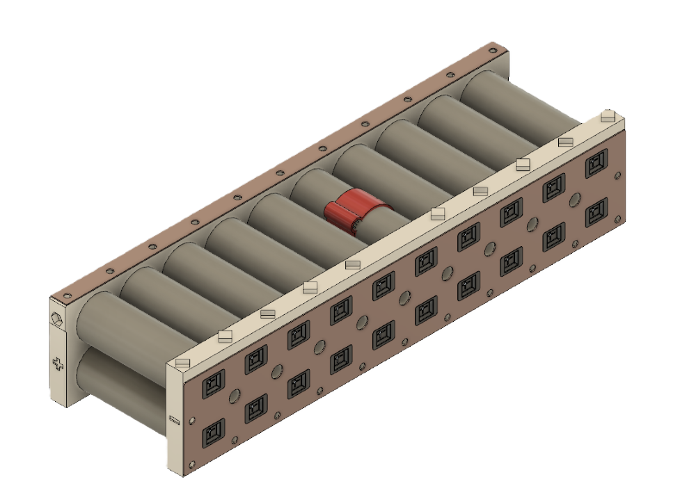 Right module
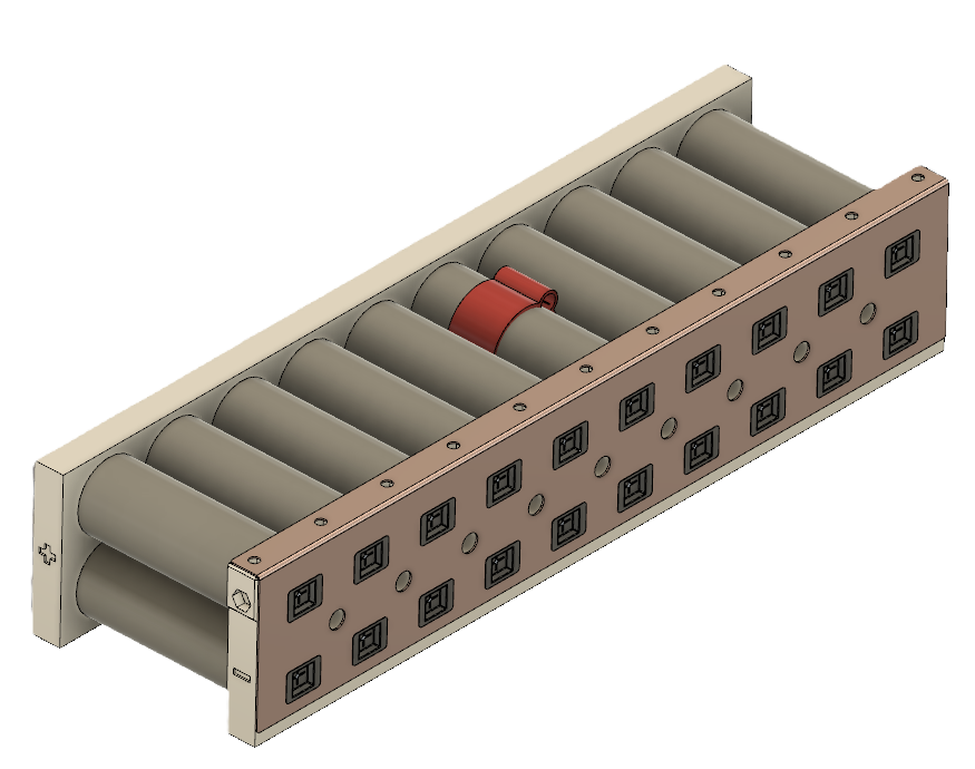 Left module
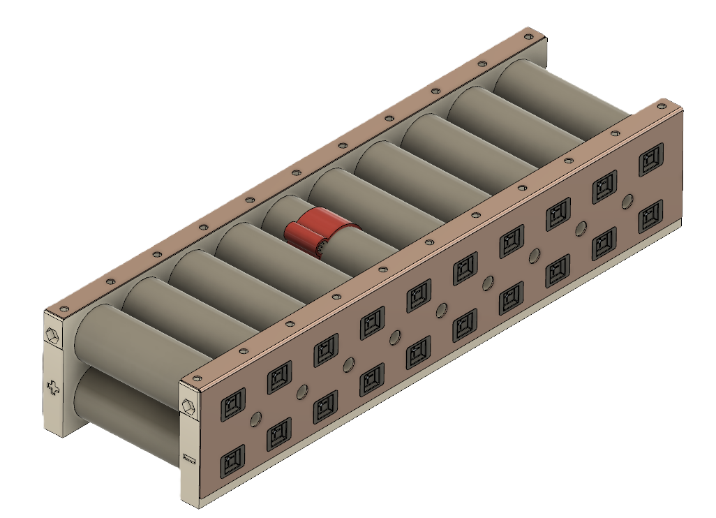 Central module
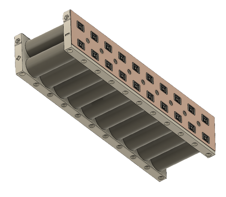 Central module. Note the holes for the lower module screw heads.
Below you can see the section of the battery. You can see the union between two modules in the central part with a 1 mm thick busbar. It’s also worth noting that precise measurements were taken for the design and as you can see, the same space has not been left between the nickel tab and the battery on both sides. This is because we try not to force the electrical connection. The battery must support and make a package with the 3D printed parts, not with the connections.
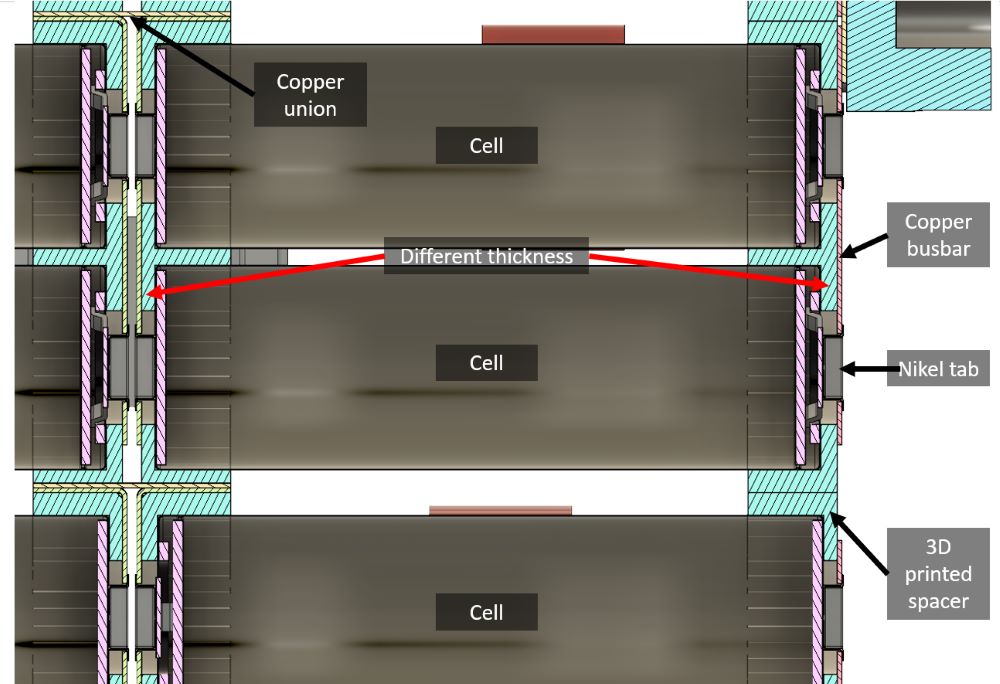 Section view of the connections between nickel tabs and cells.
Similarly, in the section below we can see how the copper connections are connected to the modules. For this purpose, M3 allen head screws are used. These screws have two functions, to ensure the electrical connection to the copper and to serve as a guide and support for the upper modules. The nuts are pressed in before assembly with an adapted soldering iron, so that they are tight and don’t turn once the screw is tightened (The nut is on the lower part of the drawing. In reality it was not like that).
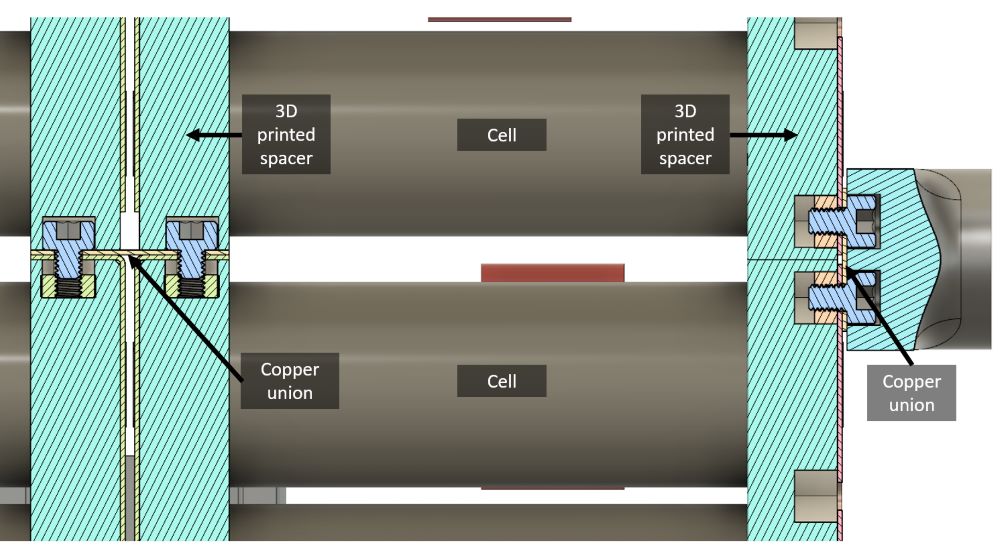 Section view of the copper connections
We tested two materials that could withstand high temperatures and had good resistance for the structure: TPU Hardness and PA HT. Both materials exhibited excellent properties for our application, however, we discovered during testing that TPU Hardness absorbed a lot of humidity, causing the piece to swell and become gummy, making it clear which material we would use.
After adjusting the printer, we proceeded with the printing using a 0.4 mm nozzle.
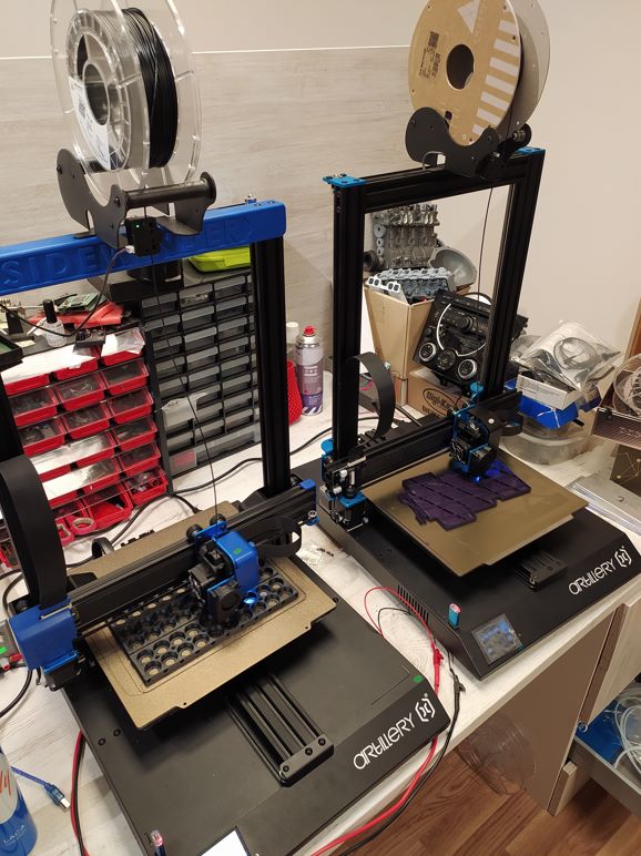 On the left, printing battery structure
Connections
Generally, lithium battery connections are made using nickel alloys combined with other metals like steel. This allows for easy soldering, although nickel has inferior conductivity compared to copper.
As I mentioned earlier, at the time of battery manufacturing, we anticipated that the inverter and motor would demand more current than they ultimately did. Therefore, we believed that nickel strips alone would not be sufficient for the connections.
We should try to use lowest amount of copper as possible because it’s expensive and heavy. We need to take care about the current that is going to flow thought the copper. If we demand 600A to the battery, each cell is going to give us 30A. We will have a current flow more or less like this:
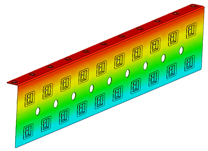 Current flow on copper plate
The problem is that it’s the first time we have designed something like this, and you always try to go with a margin that ends up being much larger than expected. We tried other suppliers but the quality did not convince us.
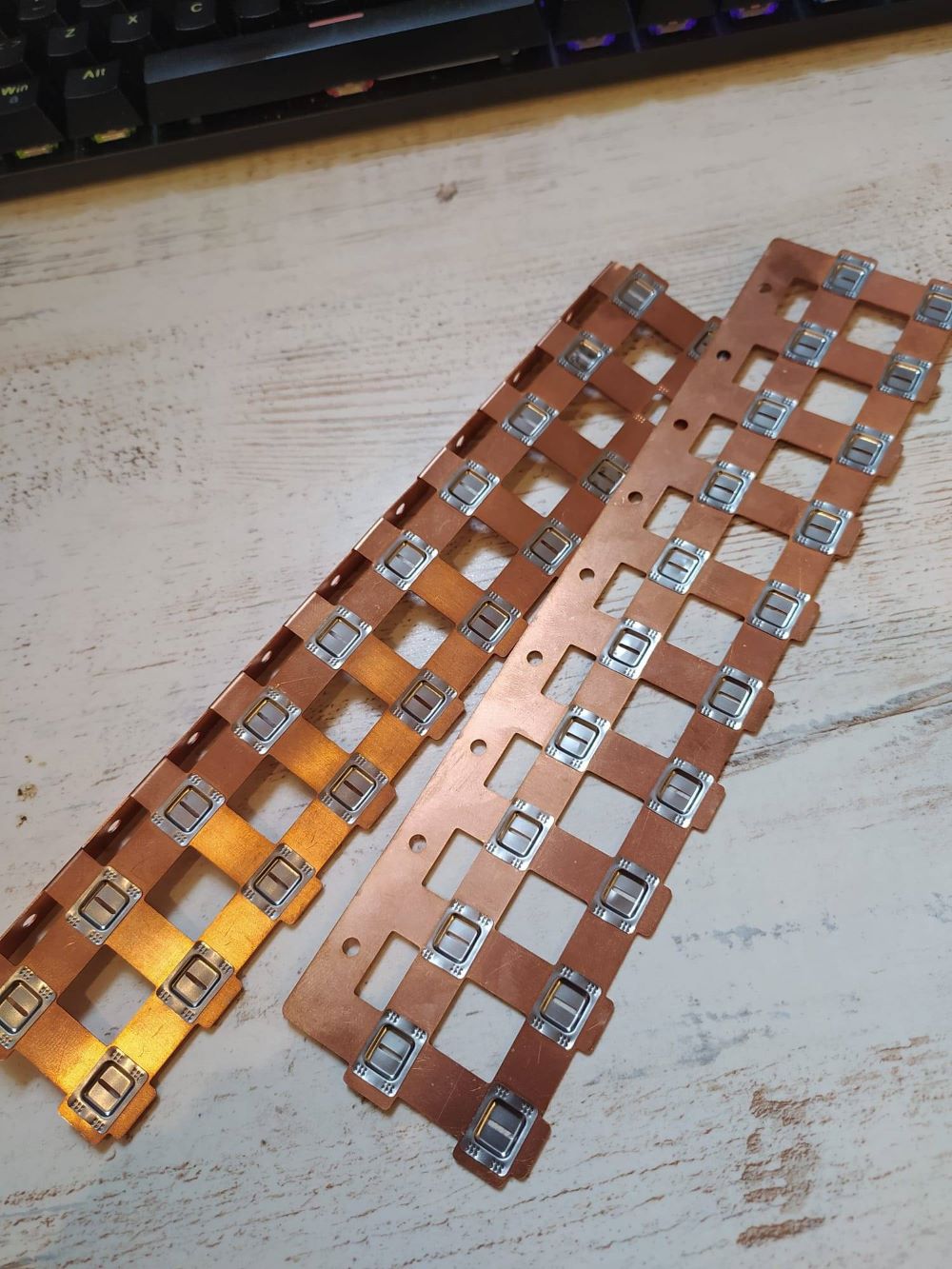 Low quality busbars. Some of the nickel tabs come off.
Our final supplier (from Alibaba) offered busbars in bare copper or nickel plated as shown below. In our case copper was more than enough. In addition, nickel plated is more expensive.
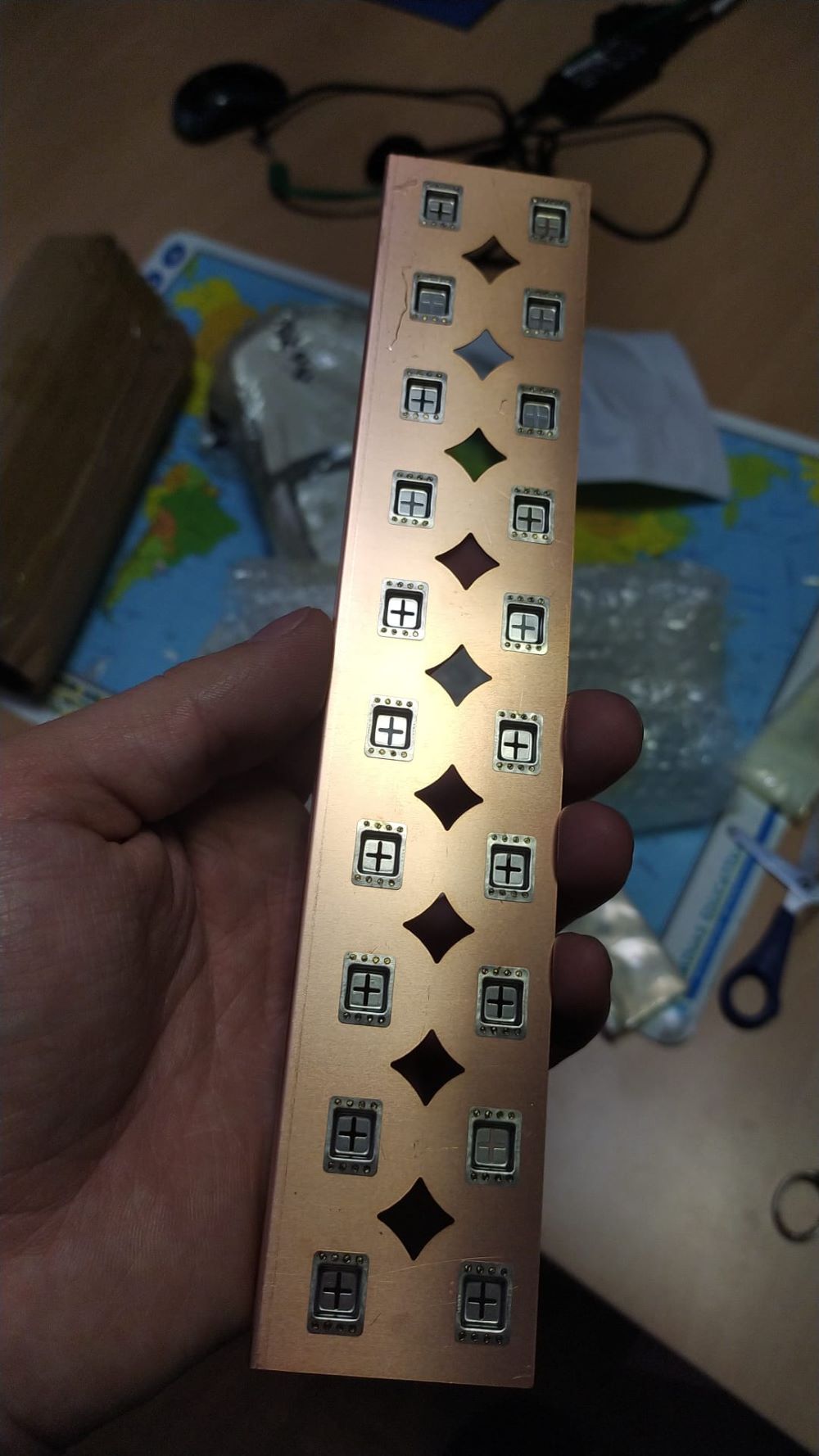 Copper busbar |
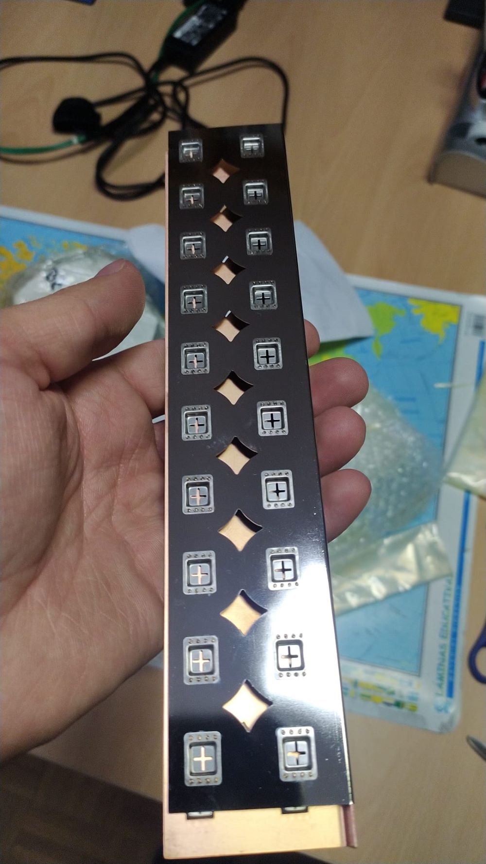 Nickel-plated busbar |
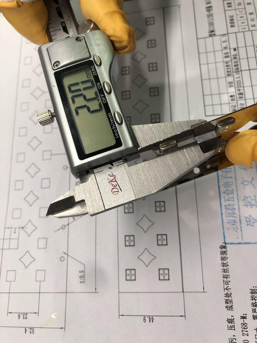 Dimensions |
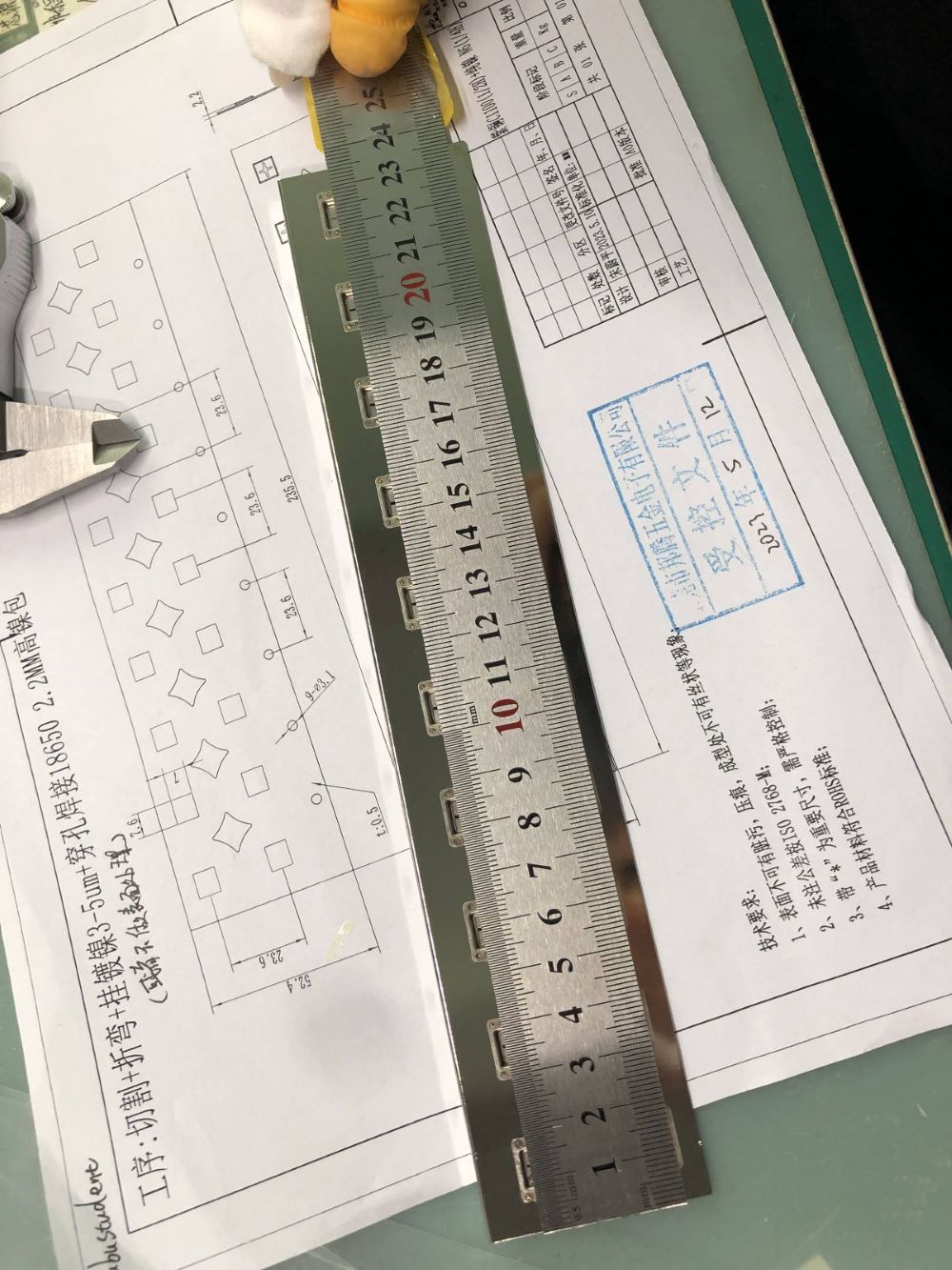 Dimensions |
As can be seen, these copper busbars feature nickel inserts of 0.15 mm. This design allows us to solder the batteries to the busbars easily. The manufacturer also offered the same busbars covered in nickel, which I assume is a treatment to prevent corrosion.
As shown above, we studied multiple battery designs before the final one. One of the main reasons was the minimum section, that is, the point at which the current is concentrated. Let’s take an example with the following design of a laser welding:
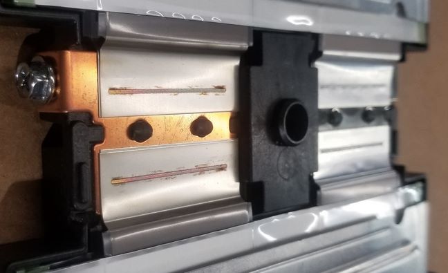 Laser welded cell
At first we might think that this welding line is insufficient. With this, I mean that the welding has not been taken to the extremes (let’s suppose that this line is the only contact area between the copper and the battery terminal). However, if we analyze it in depth we can realize that the section of the weld is much larger than the total section of the battery terminal, so this welding will never be a problem.
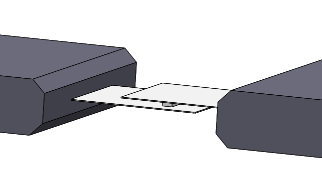 Example of laser welding. Space between terminals has been increased for clarity.
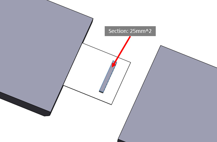 Welding section
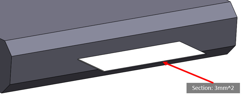 Terminal section
This is a small example to understand that we must carry out this analysis during the construction of the battery, both to avoid sections that are too narrow and concentrate too much current and to avoid the use of unnecessary material or excessive complexity that does not give us any advantage.
Connection Welding
To manufacture the battery, it’s essential to connect all the cells with a common element known as a busbar. There are different options for soldering these busbars, as discussed below:
- Solder (tin): This option is the least recommended because soldering requires the surface to be heated. As mentioned earlier, it’s not good for the cells to increase in temperature, so this option is discarded.
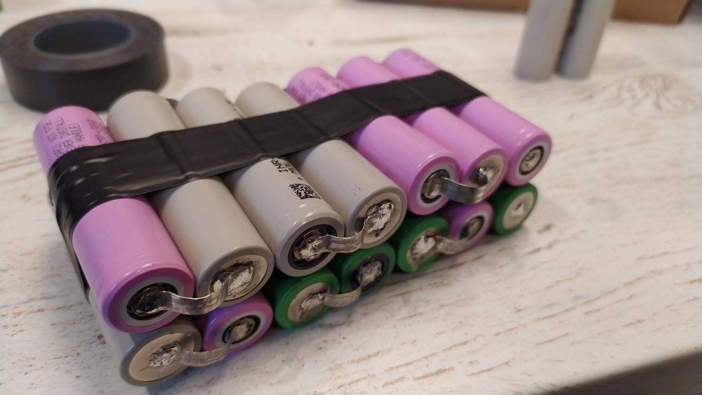 Tin soldered batteries for testing
- Laser Welding: This type of welding is the most professional and is commonly used today in vehicles and any professional production. Laser welding offers high precision and minimizes the heat-affected zone, reducing the risk of damage to the battery cells. It also enables faster production times and improved joint quality, making it a preferred method in modern battery manufacturing.
Laser welded cell
We got the help of a company to do a welding test but we don’t know if the welder’s skill was not the best or what happened, but this was the result:
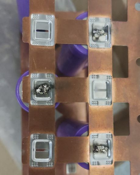 Laser welding test
Of course this is not valid for our battery.
- Spot Welding: This is the most commonly used method, especially in small vehicles and homemade batteries. Nickel strips are used to connect the cells, and the welding is performed using high current.
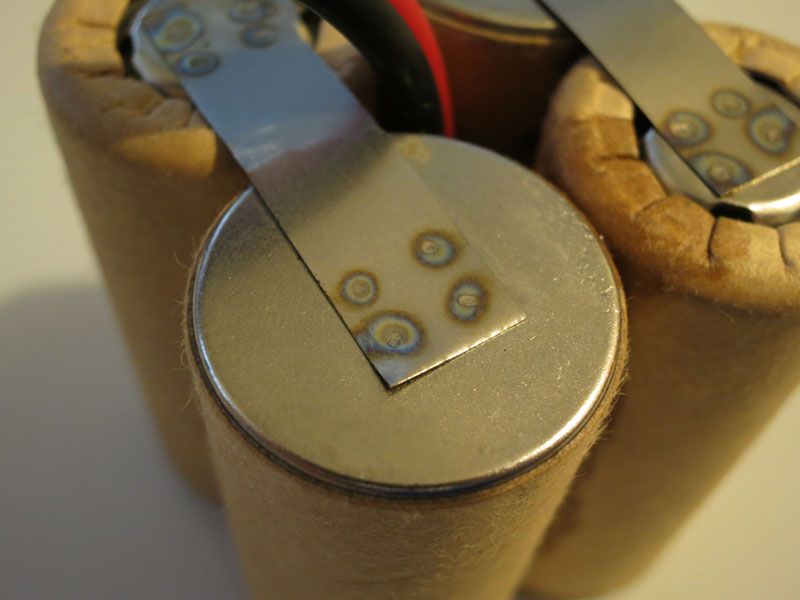 Example of spot welding |
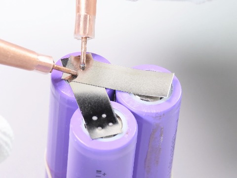 Example of spot welding |
Without a doubt, this would be the technique we would apply, both for its simplicity and effectiveness. Ultimately, the battery had a total of 8,000 spot welds.
Battery Manufacturing
Some photos of the manufacturing process of the battery:
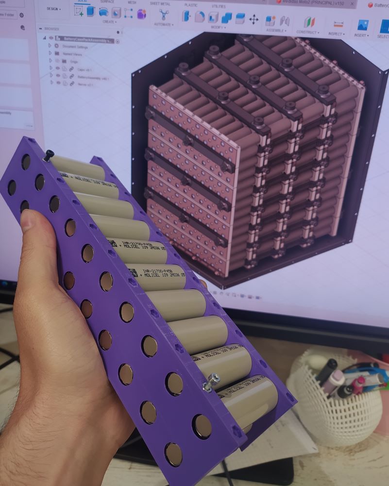 First prototype |
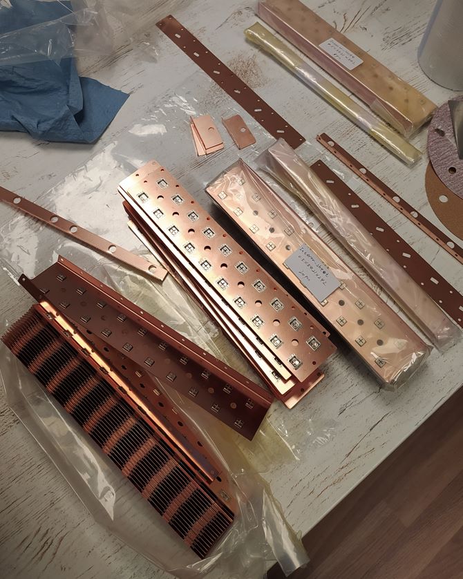 Copper busbars |
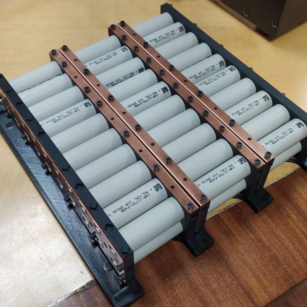 |
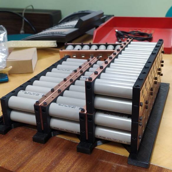 |
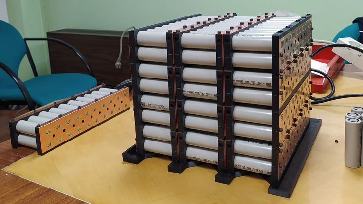 |
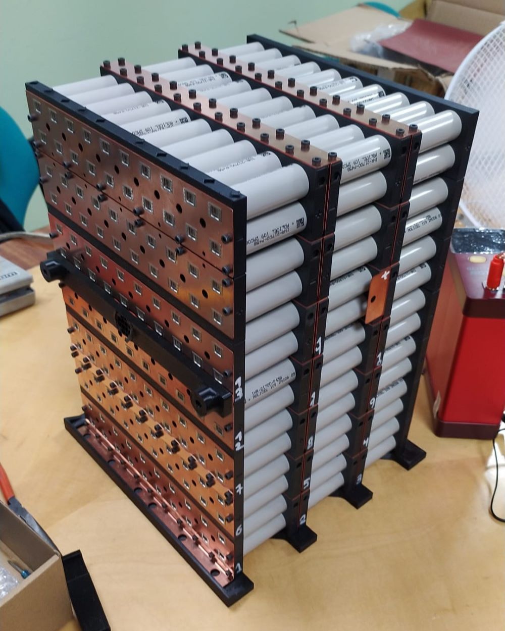 |
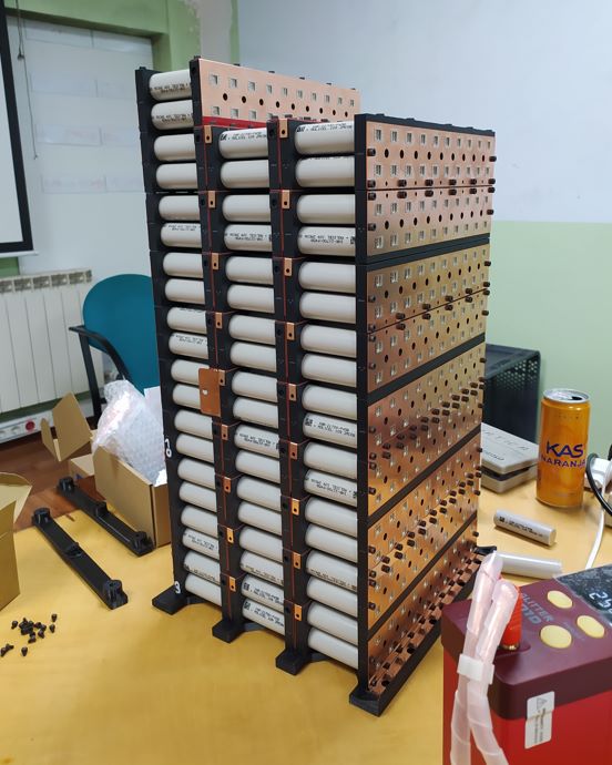 Final battery with more than 8000 spot welds |
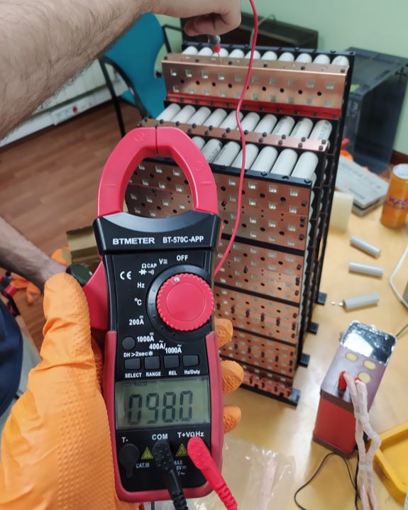 HV connections finished |
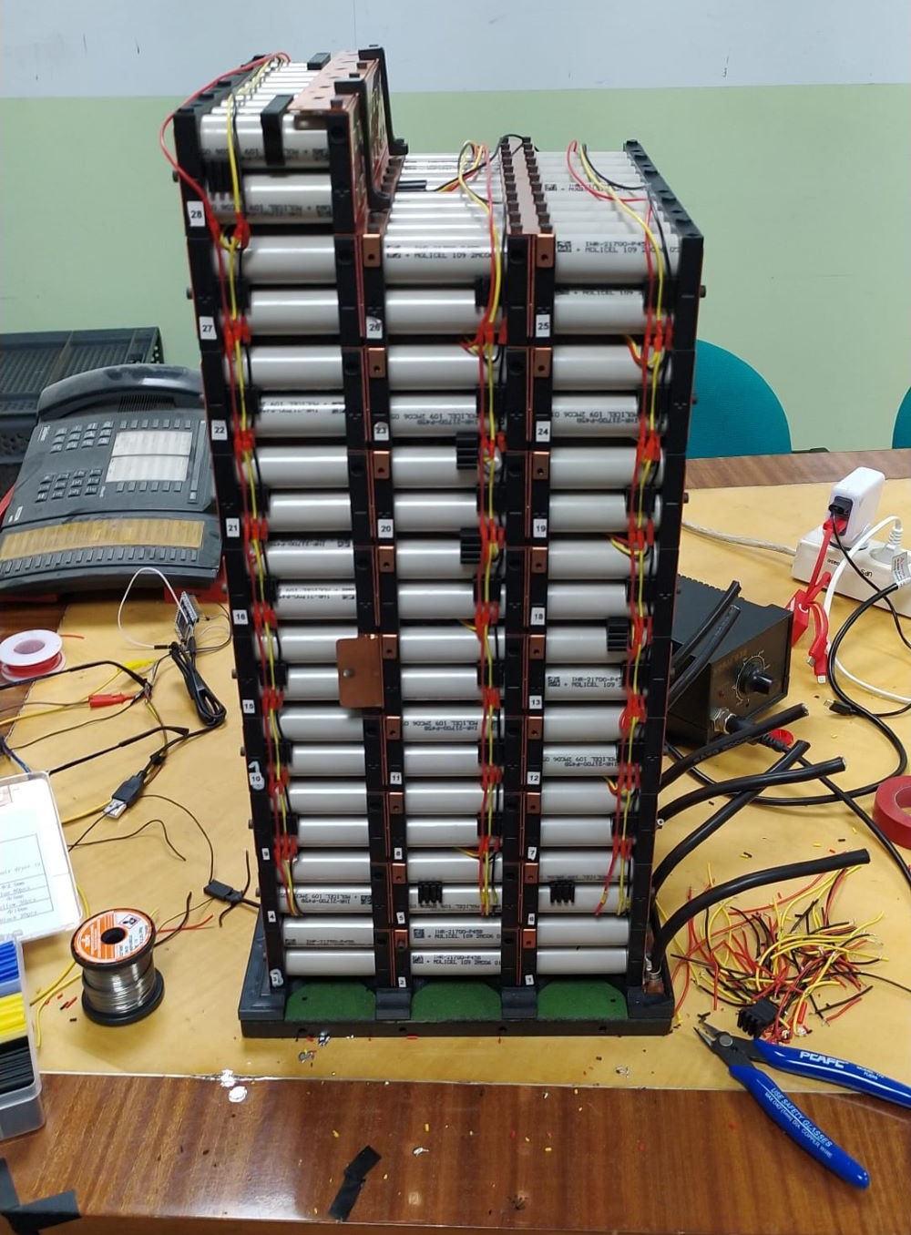 Installing temperature sensors
Battery Container
We needed a container to store the battery. We had three options for manufacturing it:
-
Machined aluminum: Probably the best option and the most rigid, but also the heaviest. We did not have the budget for this structure, so we discarded it.
-
Fiberglass/carbon fiber: Another fairly good option, but like the previous choice, it was too complex for what we were looking for, and we did not have enough expertise in working with these materials.
-
Folded sheet metal: Initially, we thought it would not be possible to manufacture a battery container from folded sheet metal. We needed a kind of cube in which we could mount the battery on a table, resting on the cube’s base, and then close it. After refining the initial idea, we decided to go with this material and technology.
For the design, we used two types of materials and two different thicknesses. The base and the top cover would be made of laser-cut and folded carbon steel with a thickness of 1.5 mm. The front and rear panels would also be made of carbon steel but with a thickness of 1 mm, reinforced with riveted ribs.
Finally, the two side panels would be made of 1 mm laser-cut aluminum. This would help reduce weight, especially since these panels did not have any folds. You might be wondering why a metallic container for storing a battery, perhaps it is not a good idea. We thought the same. To make the container insulated, we turned to one of our sponsors. In this case, we applied a layer of PVC to the entire interior of the battery container, ensuring they would be completely insulated.
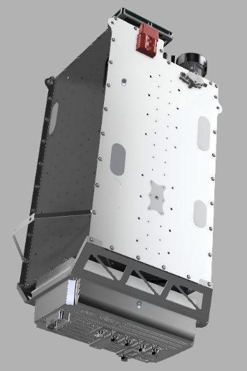 Render of battery container |
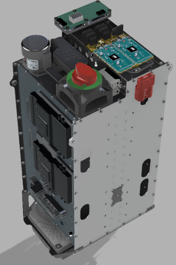 Render of battery container |
The inverter was positioned under the battery, held in place with a laser-cut aluminum folded part, near the battery and the electric motor.
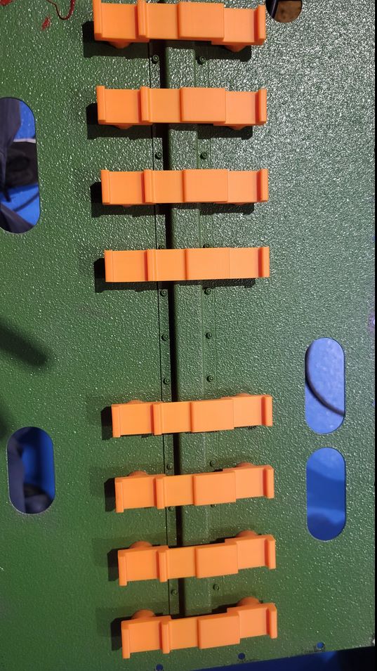 PVC insulation |
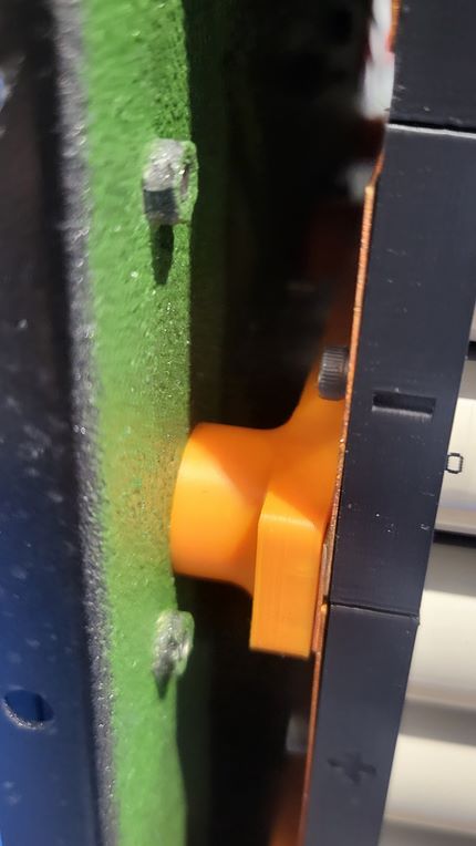 PVC insulation |
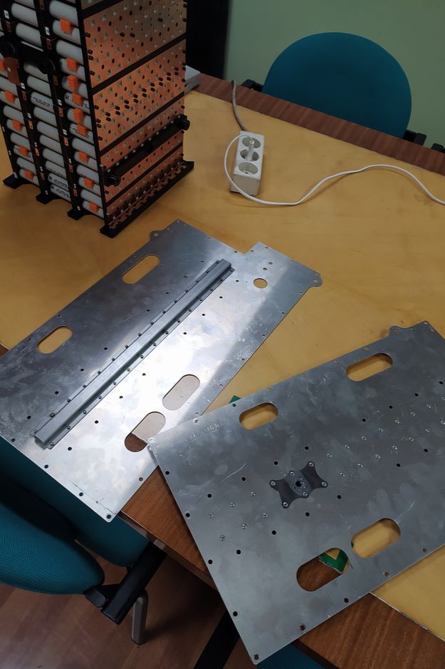 Lateral plates |
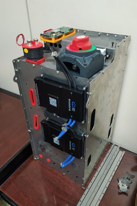 Pre-assembly |
The final conclusion we have reached is that it’s not worth making a modular battery. The probability of a cell failing is very small. In addition, there are two possibilities: the cell shorting out (the worst case scenario) since we would lose the voltage of a series and the current would flow through it, and the possibility of a cell being left open, so we would have one less cell in parallel in that series and the battery would continue to work perfectly.
Making a modular battery complicates manufacturing and increases the price, and a battery for a racing prototype like this, which will be used a few times, has small chance of breaking down if the voltages and temperatures are correctly monitored and controlled.
Other Battery Examples
Here I’m going to analyze the designs from other teams that I found making some research.
Unirioja Motostudent
I think the team didn’t race this edition but here is the battery from previous edition. It looks like it’s built with Molicel P28 cells. From my point of view, these cells are too small and covering the battery with plastic doesn’t help to cool it.
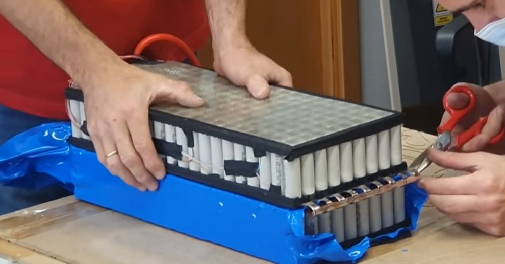 Unirioja battery
Araba Motostudent
This battery uses a Molicel P42 cells and a honeycomb structure. Probably they have a 28s 19p. This is a 117.6V with 79.8 Ah. Unfortunately their prototype got burned when they were mounting the battery.
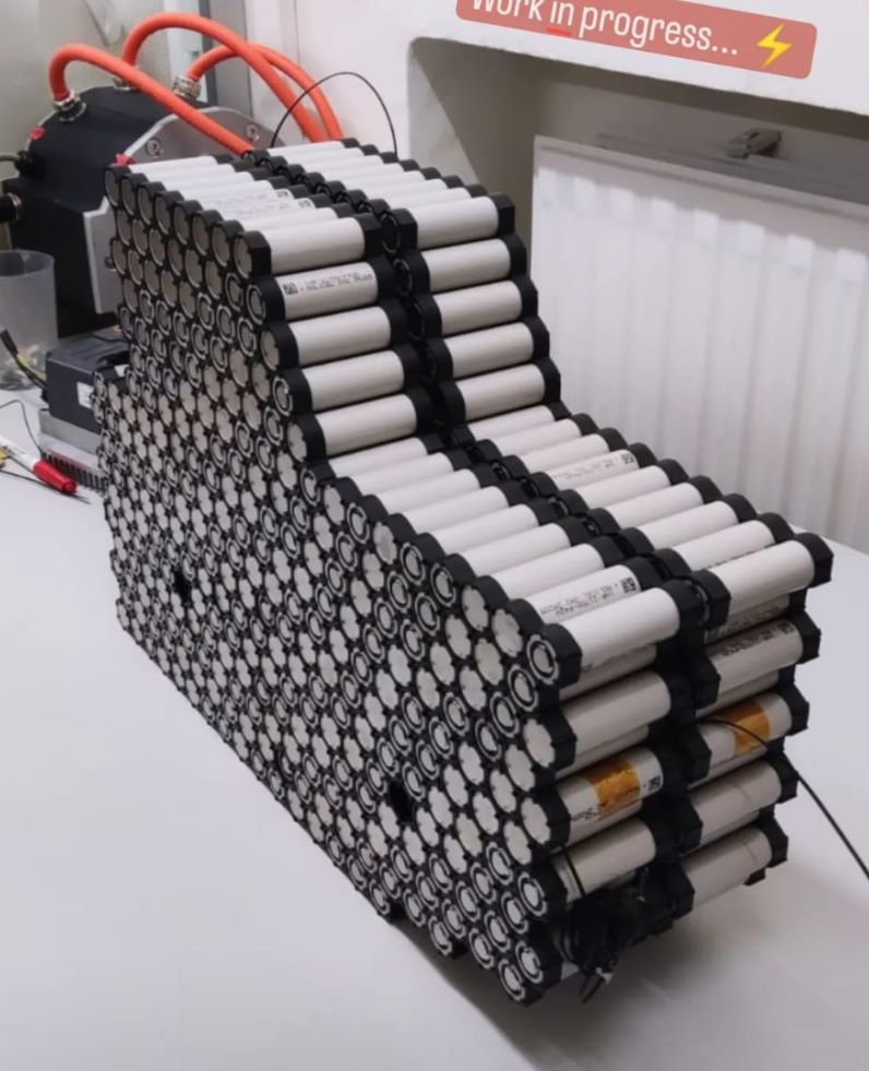 Araba motostudent battery
UMA Racing Team
This team won the past edition of Motostudent and as I have seen on some media content, they always try to hide the battery, I don’t know why. Some teams say that they use some zener diodes to fake the voltage read from Sevcon as this inverter only supports 120V. As we can see on the images, they use a LiPo cells from Melasta. It looks like they have a 30s 7p structure. This means that fully charged it has 126v at 4.2V per cell. This means that, or they use Zener diodes/another mechanism to manipulate the input voltage read by the inverter or they doesn’t charge the battery to full voltage. Another options is that they use a servo motor to apply pressure over the battery cells. Lipo battery cells need to be compressed to work correctly so perhaps when they start the race/organization measures battery voltage, they doesn’t apply pressure to the battery an as the battery voltage drops, they start pushing pressure over the battery cells.
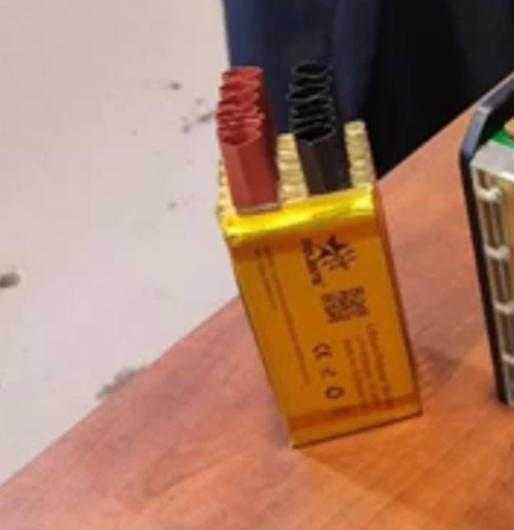 UMA Racing cells
The battery structure is quite simple, with the cells first making the parallel connections and then the series and connected between them with a copper busbars.
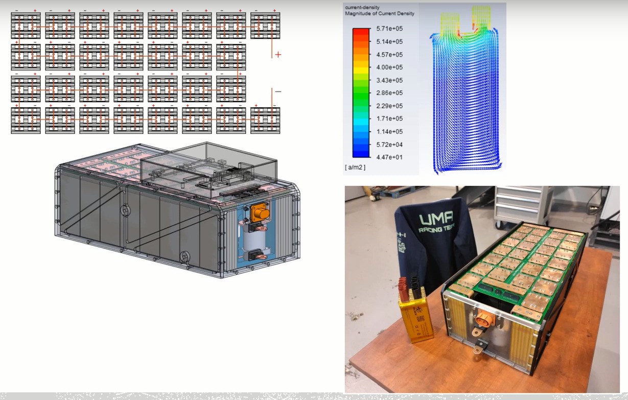 UMA battery structure
UPM Motostudent
The structure of the battery is 30s 16p with a maximum voltage of 126V and 64 Ah of capacity. They use a DANA TM4 inverter that supports a maximum voltage of 130V so they can charge the batteries until full voltage.
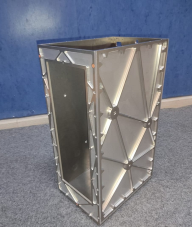 UPM battery container
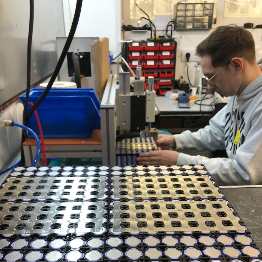 Spot welding process
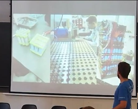 Battery structure
Charging
With a big battery, we need a big charger too if we want to charge it fast. There are multiple solutions in the market for charging lithium batteries, but not of this size. We had a sponsor that manufacture chargers and we wanted to use them for charging our battery. The problem is that the biggest charger that they had didn’t have enough voltage for our battery (117.6 V). Also, as we will see later, it was difficult and expensive to find a BMS for this voltage.
After evaluating different options, we took a decision: Use two chargers and split the battery in two blocks, not physically but logically. This means that we are going to charge the battery with two chargers with a maximum voltage of 58.8V each one, which is easier to find in addition to the BMS.
 Fronius 4045 (48V 45A 3Kw)
This chargers are designed for lead acid batteries mainly. They have a patented system23 for that batteries but is not valid for our prototype. The point is that this chargers have compatibility with other battery types such as Ni-Cd, but not Lithium (they had other series for lithium but was complex for us to connect to the BMS in a short period of time). On these chargers you can set the cell voltage that you want, for example for Ni-Cd batteries. The problem is that his cells go from 1.4 to 1.75 volts so they are not valid for our batteries (that need 4.2V per cell). We found a workaround to make it valid using it as “power supply” as on Ni-Cd mode you have steps of 0.01V.
| Fronius voltages | ||||||
| Gel | Acid | Ni-CD | ||||
| Cells | 2.3 | 2.4 | 2.35 | 2.45 | 1.4 | 1.75 |
| 1 | 2.3 | 2.4 | 2.35 | 2.45 | 1.4 | 1.75 |
| 2 | 4.6 | 4.8 | 4.7 | 4.9 | 2.8 | 3.5 |
| 3 | 6.9 | 7.2 | 7.05 | 7.35 | 4.2 | 5.25 |
| 4 | 9.2 | 9.6 | 9.4 | 9.8 | 5.6 | 7 |
| 5 | 11.5 | 12 | 11.75 | 12.25 | 7 | 8.75 |
| 6 | 13.8 | 14.4 | 14.1 | 14.7 | 8.4 | 10.5 |
| 7 | 16.1 | 16.8 | 16.45 | 17.15 | 9.8 | 12.25 |
| 8 | 18.4 | 19.2 | 18.8 | 19.6 | 11.2 | 14 |
| 9 | 20.7 | 21.6 | 21.15 | 22.05 | 12.6 | 15.75 |
| 10 | 23 | 24 | 23.5 | 24.5 | 14 | 17.5 |
| 11 | 25.3 | 26.4 | 25.85 | 26.95 | 15.4 | 19.25 |
| 12 | 27.6 | 28.8 | 28.2 | 29.4 | 16.8 | 21 |
| 13 | 29.9 | 31.2 | 30.55 | 31.85 | 18.2 | 22.75 |
| 14 | 32.2 | 33.6 | 32.9 | 34.3 | 19.6 | 24.5 |
| 15 | 34.5 | 36 | 35.25 | 36.75 | 21 | 26.25 |
| 16 | 36.8 | 38.4 | 37.6 | 39.2 | 22.4 | 28 |
| 17 | 39.1 | 40.8 | 39.95 | 41.65 | 23.8 | 29.75 |
| 18 | 41.4 | 43.2 | 42.3 | 44.1 | 25.2 | 31.5 |
| 19 | 43.7 | 45.6 | 44.65 | 46.55 | 26.6 | 33.25 |
| 20 | 46 | 48 | 47 | 49 | 28 | 35 |
| 21 | 48.3 | 50.4 | 49.35 | 51.45 | 29.4 | 36.75 |
| 22 | 50.6 | 52.8 | 51.7 | 53.9 | 30.8 | 38.5 |
| 23 | 52.9 | 55.2 | 54.05 | 56.35 | 32.2 | 40.25 |
| 24 | 55.2 | 57.6 | 56.4 | 58.8 | 33.6 | 42 |
| 25 | 57.5 | 60 | 58.75 | 61.25 | 35 | 43.75 |
| 26 | 59.8 | 62.4 | 61.1 | 63.7 | 36.4 | 45.5 |
| 27 | 62.1 | 64.8 | 63.45 | 66.15 | 37.8 | 47.25 |
| 28 | 64.4 | 67.2 | 65.8 | 68.6 | 39.2 | 49 |
| 29 | 66.7 | 69.6 | 68.15 | 71.05 | 40.6 | 50.75 |
| 30 | 69 | 72 | 70.5 | 73.5 | 42 | 52.5 |
| 31 | 71.3 | 74.4 | 72.85 | 75.95 | 43.4 | 54.25 |
| 32 | 73.6 | 76.8 | 75.2 | 78.4 | 44.8 | 56 |
| 33 | 75.9 | 79.2 | 77.55 | 80.85 | 46.2 | 57.75 |
| 34 | 78.2 | 81.6 | 79.9 | 83.3 | 47.6 | 59.5 |
| 35 | 80.5 | 84 | 82.25 | 85.75 | 49 | 61.25 |
| 36 | 82.8 | 86.4 | 84.6 | 88.2 | 50.4 | 63 |
| 37 | 85.1 | 88.8 | 86.95 | 90.65 | 51.8 | 64.75 |
| 38 | 87.4 | 91.2 | 89.3 | 93.1 | 53.2 | 66.5 |
| 39 | 89.7 | 93.6 | 91.65 | 95.55 | 54.6 | 68.25 |
| 40 | 92 | 96 | 94 | 98 | 56 | 70 |
We have a 28s battery but the charger is going to work on a 14s battery. This means that we need 4.2V * 14 = 58.8 V.
58.8 / 35 = 1.68V. We can set the charger to a Ni-Cd battery with 35 cells and 1.68V per cell.
If for example we want to charge the battery with 90A (current limit), on the charger we should input the battery Ah. Then, we must set 900Ah as battery capacity.
The charger will work as a power supply, limiting the charging current when the voltage is below the configured and limiting the voltage when it reaches the established one. When the battery stops consuming current and it’s at the configured voltage, the charger will consider the battery charged, stopping the process.
On the other hand, the BMS will perform its balancing function during the charging process, and when the cells have reached the maximum voltage, it will cut off the current coming from the charger, and the charger will stop too. This means that the charger may cut off first, or the BMS may cut off first, but we will not exceed the voltage (let’s say we have 2 protection elements).
These Fronius chargers have isolated AC and DC circuits. This means that we could charge the battery with both chargers having it connected to the main poles. Even so, we include a disconnector to cut the main poles during the charging process.
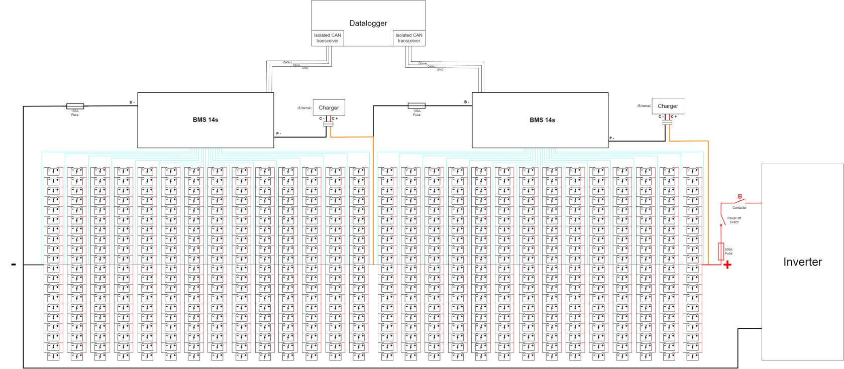 Charging system
There are two tabs in the middle of the battery. HV GND is the GND for the first charger. One of this tabs is the positive. The other tab is the GND for the second charger and the HV positive is also the positive for the second charger.
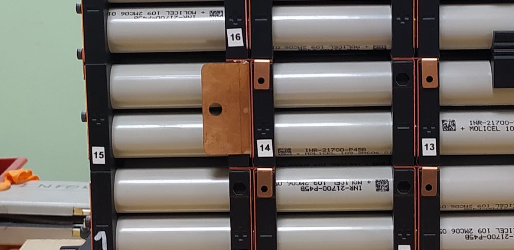 Internal charging terminal
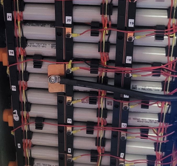 Charging terminal connected
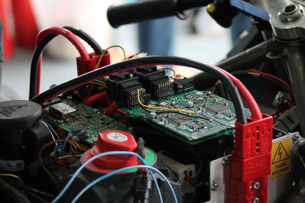 Battery charging process. Note both chargers connected at the same time.
BMS (Battery Management System)
Introduction
Lithium batteries are unstable and tend to be unbalanced. This means that they have different internal resistance between cells and one cell will charge/discharge before another one.
Here is when the BMS comes in. The BMS is a system designed to monitor and protect the batteries. They have mainly 4 goals:
- Temperature protection: Cells must work in a range of temperature specified by the manufacturer. If they work outside that range, they can be dangerous, short their lifespan and more. There are some BMS that have heater outputs to heat the battery when it’s too cold.
- Current protection (overcurrent protection): Cells are designed to hold a specified maximum current on charge and discharge. The BMS protects them from high current peaks.
- Voltage protection (overvoltage/undervoltage protection): Cells must work between a specific voltage range defined by the chemistry and manufacturer.
- Balance: As the cells tend to be unbalanced, the BMS must be able to balance the difference between the battery cells.
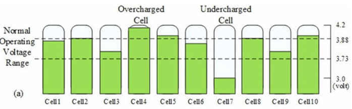 Example of unbalanced battery24
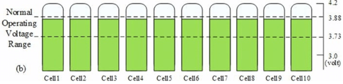 Example of balanced battery24
Balancer
The balancer is used to balance the voltage of the cells. There are two types of balancers:
Passive balancers
They are simple and cheap. These balancers use resistors to convert energy into heat and be able to discharge the most charged cells. Normally the balancing current is low on this type of balancers or they need a big heat exchanger / heat skin to dissipate heat.
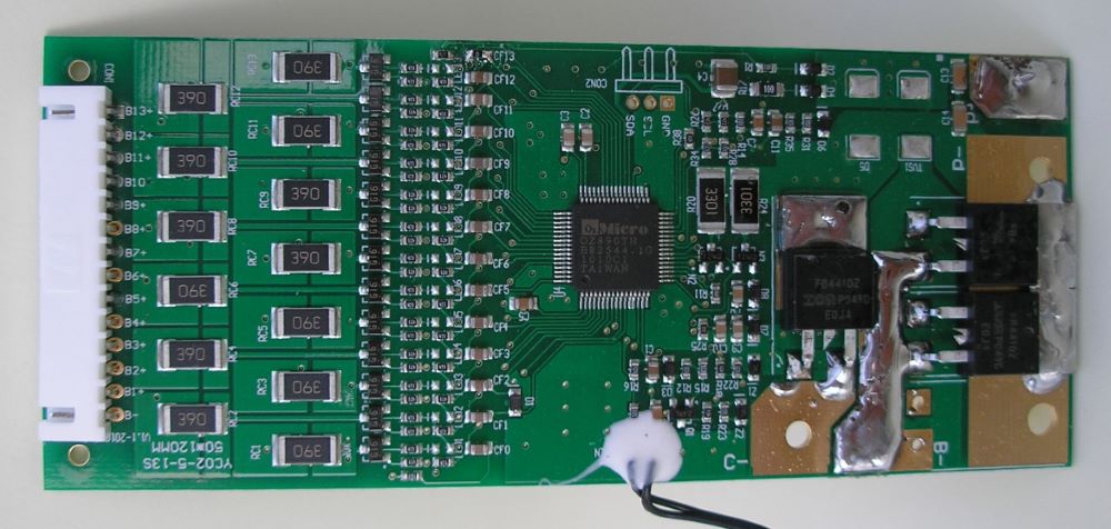 Example of BMS with passive balancer
Active balancers
These balancers send current between the battery cells so the energy is not lost. This technology is more complex and expensive. There are multiple methods for achieve the active balancing, but usually they allow a higher balancing current.
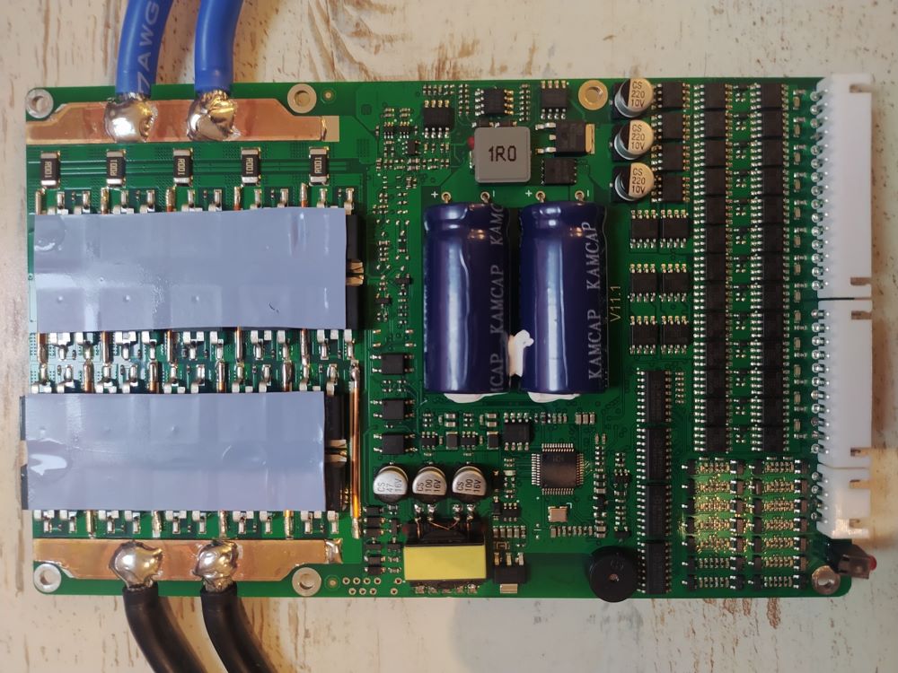 JK BMS with active balancer
BMS Comparison
We needed a BMS for the prototype. Our specifications were a charge current higher than 90A, highest balancing current, CAN or UART communication and 14S or more. Also we were looking for the cheapest and lightest hardware. After hours and hours searching we got all this information to compare:
| Brand | Model | Charge (A) | Discharge (A) | Type | Balance (mA) | Communication | Series | Voltage | Temp sensors |
| Ennoid | Gen 1 | 500 A | 500 A | Passive | 125 | CAN | 5-18 | 30-150 | 9 |
| Fox | FoxBMS2 | Contactor | Contactor | Passive | 55 | UART | 3-18 | 16-90 | 8 |
| DieBieEngineering | DieBieMS | 30 A | 70-100 A | Passive | - | CAN | 3 - 12 | 12-54 | 2 |
| Speedict-Neptune | 15 | 39 A | 178 A | Passive | - | Bluetooth | 10-15 | 42-63 | 1 |
| 20 | 39 A | 250 A | Passive | - | Bluetooth | 12-20 | 50-84 | 1 | |
| Electrodacus | DMPPT450 | 100A | 100A | Passive | - | UART | 3-8 | 12-24 | 2 |
| REC BMS | REC 2Q | 500 A | 500 A | Passive | 900 | CAN | 4-240 | 14-800 | 4 |
| BatteryHookup | BMS | 30 A | 30 A | Passive | 50 | - | 3-20 | 12-72 | 1 |
| Orion | Jr 2 | 1000 A | 1000 A | Passive | 150 | CAN | 1-16 | 10-60 | 3 |
| Lithiumbalance | i-BMS15 | 100 A | 150 A | Passive | 200 | CAN | 8-15 | 17-60 | 10 |
| ANT | 10-32S | 380 A | 380 A | Passive | 100 | Bluetooth | 10-32 | 20-150 | 2 |
| GreenBikeKit | BMS | 15 A | 120 A | Passive | 60 | Bluetooth | 4-15 | 12-60 | 2 |
| MaxkGo | MaxKGo | Enoid copy? | - | - | - | - | - | - | - |
| BesTech | HCX-D575 | 120 A | 120 A | Passive | 250 | CAN | 12-28 | 44-120 | 7 |
| Minetals | 16S100A | 100A | 100A | Passive | - | UART, CAN | 15-16 | 55-60 | 2 |
| HELTEC | Relay smart | 200A | 500A | Passive | 60 | UART, CAN | 25-32 | 92-120 | 4 |
| JKBMS | B2A20S20PR | 200 A | 200 A | Active | 2000 | CAN, RS485 | 8-20 | 33-84 | 2 |
| DalyBMS | 20S M | 150 A | 75 A | Passive | 100 | Bluetooth | 3-24 | 12-100 | 1 |
| LTT POWER | 15S | 100 A | 120 A | Active | - | Bluetooth | 10-15 | 42-63 | 1 |
| ALL CELL | - | - | - | - | - | CAN | - | 60-150 | - |
| SEPLOS | 48V 200A | 200 A | 200 A | Passive | 150 | CAN | 14 | 60 | 1 |
| LTW | LTP24S009 | 200 A | 200 A | Passive | - | - | 4-24 | 16-100 | 1 |
| HUB E | Daly copy | 50 A | 100 A | Passive | 30 | - | - | - | - |
JKBMS
After reviewing all the options, our best choice was the JKBMS. This BMS has CAN, active balancer of 2A and good price and size. We selected the model B2A20S20PR with 20S and 200A. We are not going to use this BMS for discharge through it. We will only charge through it and monitor the cells with it during discharge.
Fortunately this BMS met our expectations. We mounted 2 units in our battery pack and configured it through Bluetooth connection.
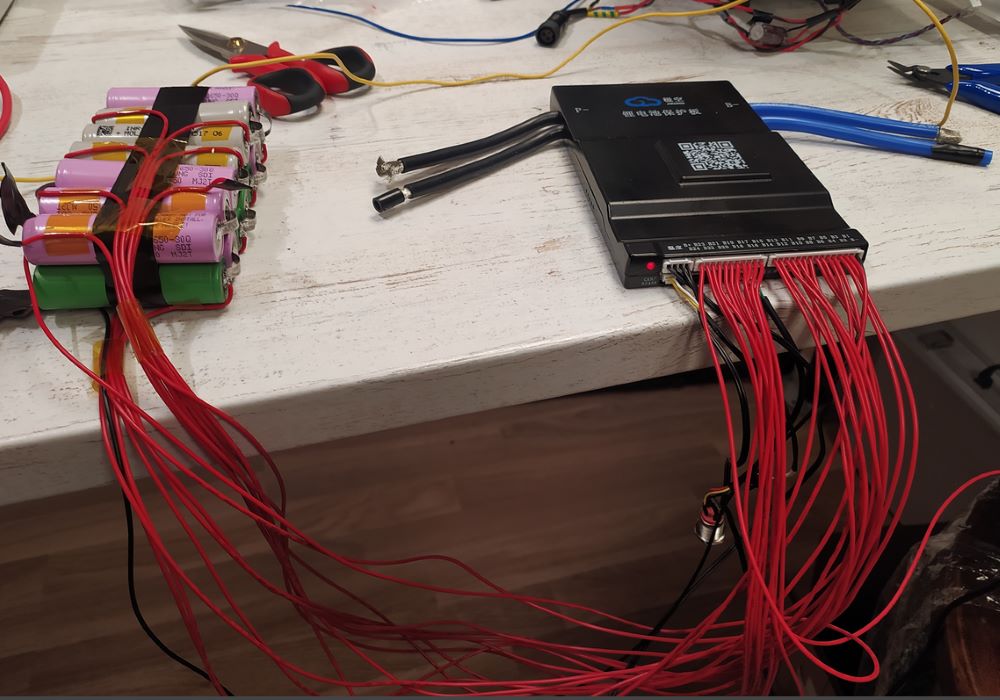 JKBMS test
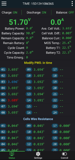 JKBMS android app for monitoring and configuration
Note that it’s important to configure both the chargers and the BMS as accurately as possible. The chargers have an option to enter the length of the charging cable in order to measure its resistance and to be able to perform a more precise calculation of the voltage. In the same way, the BMS have an option to configure the length of the balancing wires. After these adjustments, this charging system worked perfectly for us. The battery was completely balanced and everything worked perfectly.
CAN Decoding
To program the datalogger and the BMS electronics we need to collect data from the JKBMS. It has a CAN interface through which each BMS sends the following data:
| CAN ID | Data | Position | Length (bits) | Period |
| 0x04F4 | Maximum cell voltage | 0 | 16 | 100 ms |
| 0x04F4 | Maximum voltage cell number | 16 | 8 | 100 ms |
| 0x04F4 | Minimum cell voltage | 32 | 16 | 100 ms |
| 0x04F4 | Minimum voltage cell number | 48 | 8 | 100 ms |
For example, the message:
0x04F4 8C 0A 05 92 09 08 XX XX
Can be decoded25 as:
| Data | Hex value | Value |
| Maximum cell voltage | 8C 0A | 2700 mV |
| Maximum voltage cell number | 05 | 8 |
| Minimum cell voltage | 92 09 | 2450 mV |
| Minimum voltage cell number | 08 | 8 |
JKBMS also sends different events / alarms but we are going to control everything with our microcontroller so we don’t need it.
Powertrain 🚀
Let’s start talking about probably the most complex part of building an electric motorbike. Or at least, the most difficult part for making it perform. There are three main parts on an electric vehicle powertrain:
- Battery
- Motor
- Inverter
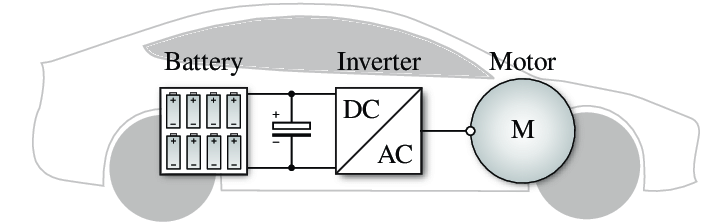
I have previously talked about batteries and the development process thereof, so in this section I will focus on the motor and inverter, two of the most complex parts to understand.
Motor
Introduction
If you are reading this, you probably know what is a motor. Let’s take a look about what kind of motors we can find.
Since I participated in the previous edition and it also served as part of the learning process, I will also talk about the motor from the previous edition, comparing the differences between the two and at the same time assuming the similarities, treating them as similar. To make it clear to the reader, I will refer to the motors as:
- ENGIRO: Previous edition motor.
- ME1616: Current edition motor.
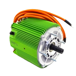
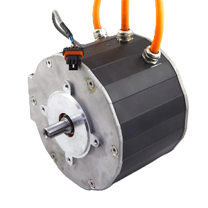
Types of Electric Motors
The first thing we must be clear about is that there are many types of electric motors. Each one has its advantages and disadvantages, making them ideal for different applications. Below we can see an incomplete diagram of the types of motors that exist and their classification. For the purpose of this post, this will be enough.
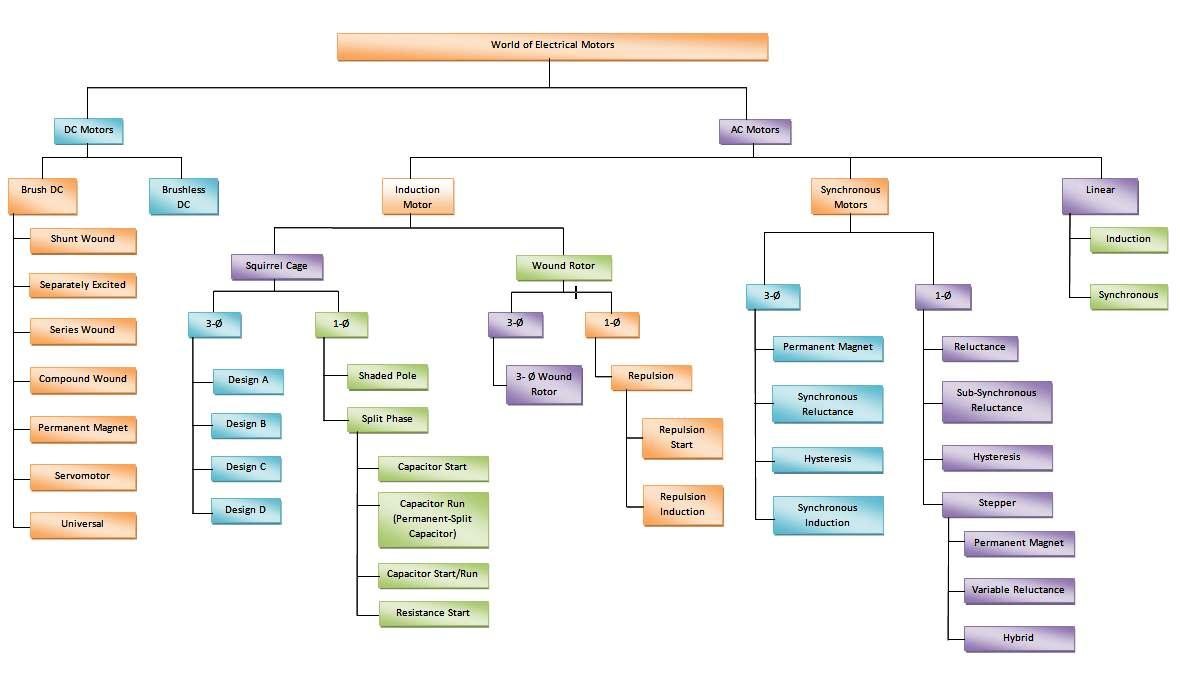 Types of electric motors26
In our case, the motor is provided by the organization. All teams have the same motor, and it’s a sealed component that cannot be modified. It’s checked after the competition, so no internal modifications can be made. Nonetheless, it’s crucial to have a solid understanding of motors to comprehend their behavior and program them effectively.
General concepts
Cooling
An electric motor is a thermal machine with efficiency. It has an energy input (electricity) that transforms into an energy output (mechanical). In this process, there is efficiency, meaning part of the input energy is lost or dissipated as heat between others. Considering that we are dealing with a competition motorcycle, all components must operate at peak performance, making heat dissipation vital.
There are two types of cooling:
-
Air-cooled: These motors typically have an outer heatsink to increase the surface area exposed to air, enhancing cooling. In this case, the ENGIRO motor is air-cooled.
-
Liquid-cooled: These motors have an internal circuit that allow liquid to flow inside the casing to absorb heat and extract it. They require a radiator and a pump to circulate the liquid within the system. The ME1616 motor is an example of a liquid-cooled motor.
Initially, a liquid-cooled motor should be more efficient in terms of heat dissipation (though, as we will see, this was not the case here). However, it has some disadvantages, such as manufacturing complexity, added weight (due to the coolant) and system complexity as a water pump and radiator are needed to complete the circuit.
Below is a schematic of the water circuit. The fluid circulates through the cooling system. When the fluid reaches the motor, a temperature exchange occurs between the hot motor casing and the cold fluid, heating the fluid. Once this fluid reaches the radiator, an inverse heat exchange occurs. The hot fluid circulates through the radiator and exchanges heat with the cooler air. After this, the fluid pump is ideally located in the cold area of the circuit.
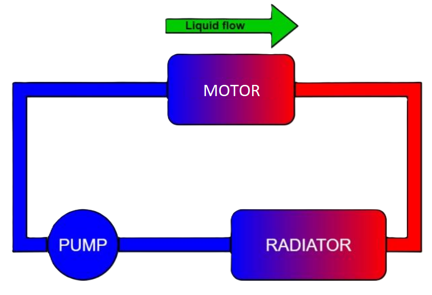 Suggested cooling circuit
It is important to note that if you wish to use the same liquid cooling circuit for both the motor and the inverter, the inverter should be positioned before the motor. This configuration ensures that the coolant, which has a lower temperature after passing through the radiator, first cools the inverter. Generally, the maximum operating temperatures of motors are higher than those of inverters. If we were to reverse this arrangement, the coolant exiting the motor would raise the temperature of the inverter. To be more specific, the maximum operating temperature of the previously mentioned motors can range between 100°C and 120°C. In contrast, the maximum operating temperature for the Sevcon Gen4 Size 6 inverter is 75°C. If the temperature rises to 85°C, the controller will deliver 0% of its power, making it crucial that we do not install it in reverse order.
Correct installation of the inverter and motor in the cooling system.
Encoder
The encoder is a measurement device responsible for determining the position of the rotor at a specific moment. It’s used to calculate when the magnetic field will be generated from the rotor to the stator. There are three main types of encoders used in PMSM motors:
- AB encoder: This encoder is primarily used in induction motors and is optimized for accurately measuring speed. However, it’s not relevant for our application.
- UVW encoder: This type of encoder is designed to determine the rotor’s position, prioritizing its rotational speed. It has three pulses that are phase-shifted by 120 degrees with a 50% duty cycle. This encoder is expected to produce one pulse for each electrical cycle of the motor.
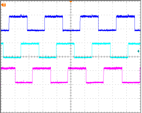 Graph of a UVW encoder measured with an oscilloscope.
- Sin/cos encoder: This type of encoder provides two signals: SIN and COS. These signals are phase-shifted by 90 degrees, with the cosine signal typically leading the sine signal during normal rotation. This encoder allows for precise knowledge of the rotor’s exact position at all times. It’s expected to generate sine and cosine waves for each mechanical revolution of the motor.
By using sin/cos encoders, applications can achieve higher precision in control and feedback, which is crucial for optimizing performance in electric motors. This encoder type is favored in high-performance applications due to its ability to provide continuous position information and improved resolution compared to other encoder types.
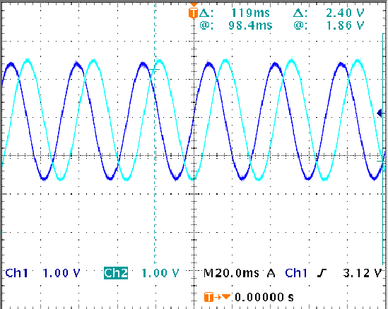 Graph of a sin/cos encoder measured with an oscilloscope.
Encoder Hardware
Focusing on sin/cos encoders, these encoders have a magnet on the rotor. This magnet generates a magnetic field with each revolution, which is then read and interpreted by the encoder chip. Some encoders convert the analog sine and cosine signals into digital signals, transmitting them via a bus such as SPI. However, in our case, the signal is directly interpreted by the inverter.
It’s important to note that these types of signals are very susceptible to interference due to their low voltage. Therefore, it’s crucial to properly shield the cable running from the motor to the inverter and to keep it as short as possible to minimize potential disruptions. By ensuring that the encoder hardware is correctly implemented, the overall performance and reliability of the motor control system can be significantly enhanced, leading to better efficiency and responsiveness in competitive settings.
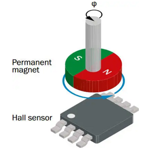 Sin/cos encoder |
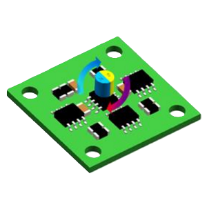 Sin/cos hardware |
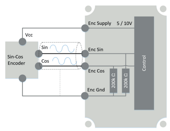 Sevcon Gen4 encoder connection
With this encoder, the inverter knows the exact position of the rotor relative to the stator at all times. This setup ensures precise control and monitoring of the motor’s performance in a competitive electric motorcycle context.
How a Permanent Magnet Motor Works
Note: Everything mentioned below refers to the ENGIRO and ME161627 motors.
As indicated in the datasheets (which can be found later), the motor provided by the organization is a “Permanent Magnet Synchronous Machine” (PMSM).
Main Components
-
Rotor: This is the moving part of the motor, serving as the motor’s shaft. In this rotor, the permanent magnets are embedded, and there is a small air gap between the rotor and stator.
-
Stator: The outer part of the motor, which contains the windings, the external casing, and the cables supplying power to the motor.
Advantages of PMSM
Permanent magnet motors are ideal for applications like these because they require minimal maintenance. The only contact point between the rotor and stator is through the bearings, meaning there are no additional wear parts that could cause issues, unlike brushed motors that experience wear and require constant maintenance.
Power Supply
These motors are powered by three-phase alternating current (AC). They have three phases through which they are supplied with a waveform, as illustrated below:
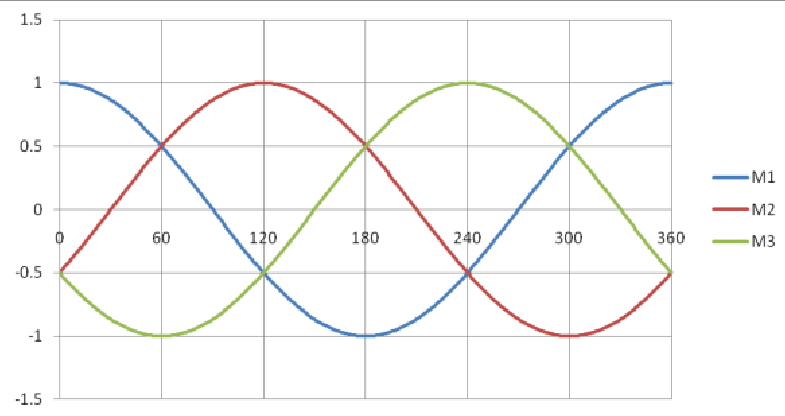 Example of 3 phases
As we can see, there is a 120 degree phase shift between each of the three phases.
In synchronous motors, the electrical frequency of the power supply and the mechanical speed of the rotor are always the same. This is the main difference compared to induction motors, where these two factors are slightly different. In induction motors, a phenomenon known as “slip” occurs due to the difference in speed between the rotor and the generated magnetic field (the phase shift), which induces a magnetic field in the rotor, transferring energy to it.
 Induction motor
In the case of PMSMs, the rotor permanently retains energy through its embedded magnets, meaning the frequency of the motor’s operation is synchronized with the rotor’s rotational speed.
Key Characteristics
There are two key characteristics that determine the behavior and application of these types of motors (among many others), which are interrelated:
Pole pairs: As mentioned earlier, the rotor contains magnets that generate a magnetic field. Each of these magnetic fields is considered a pole, and they always come in pairs, which is why we refer to them as pole pairs.
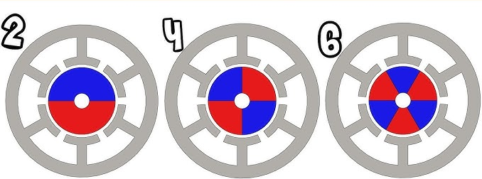 Pole pairs28
The number of pole pairs in a motor directly influences its torque and maximum revolutions. Specifically, the following points can be highlighted:
-
Torque production: More pole pairs generally result in higher torque. This is because each pole pair contributes to the motor’s ability to generate rotational force. The torque is proportional to the current flowing through the stator windings and the magnetic field produced by the rotor’s magnets.
-
Maximum RPM limitations: Conversely, an increase in pole pairs leads to a reduction in maximum revolutions per minute (RPM). This limitation arises because the inverter driving the motor has a maximum switching frequency for its transistors or IGBTs. Each cycle of the AC waveform corresponds to a complete rotation of the magnetic field, and with more pole pairs, the motor must operate at lower speeds to maintain synchronization between the rotor and stator fields.
This relationship is crucial for designing motors for specific applications, as it balances the need for torque against the desired operating speed.
Slots: There are tables with the relation of slots and pole pairs. The reason for all this is beyond the scope and intention of this post but you can consult the book “Design of Brushless Permanent-Magnet Motors” if you want to know more information on the subject.
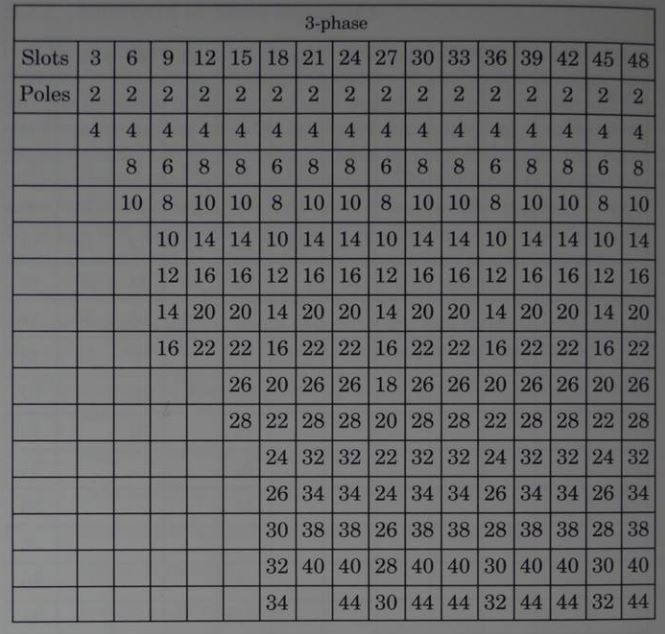 Slots vs poles29
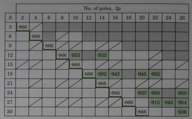 Slots vs poles29
So far, everything is relatively simple. The only problem is that we have not covered one of the most important parts, nor have we taken it into account. After hours of searching, I realized that there are two types of permanent magnet motors. This characteristic greatly affects the programming of the inverter, as we will see later:
- SPM (Surface Permanent Magnet): On these motors, magnets are pasted on the outside part of the rotor. These motors are more simple and cheaper.
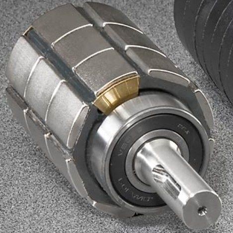 Example of SPM
However, these motors do not usually rev as high due to the possibility of the rotor spinning and the magnets being released.
- IPM (Interior Permanent Magnet): These motors have the PM embedded inside the rotor. They are more expensive but can get higher RPM.
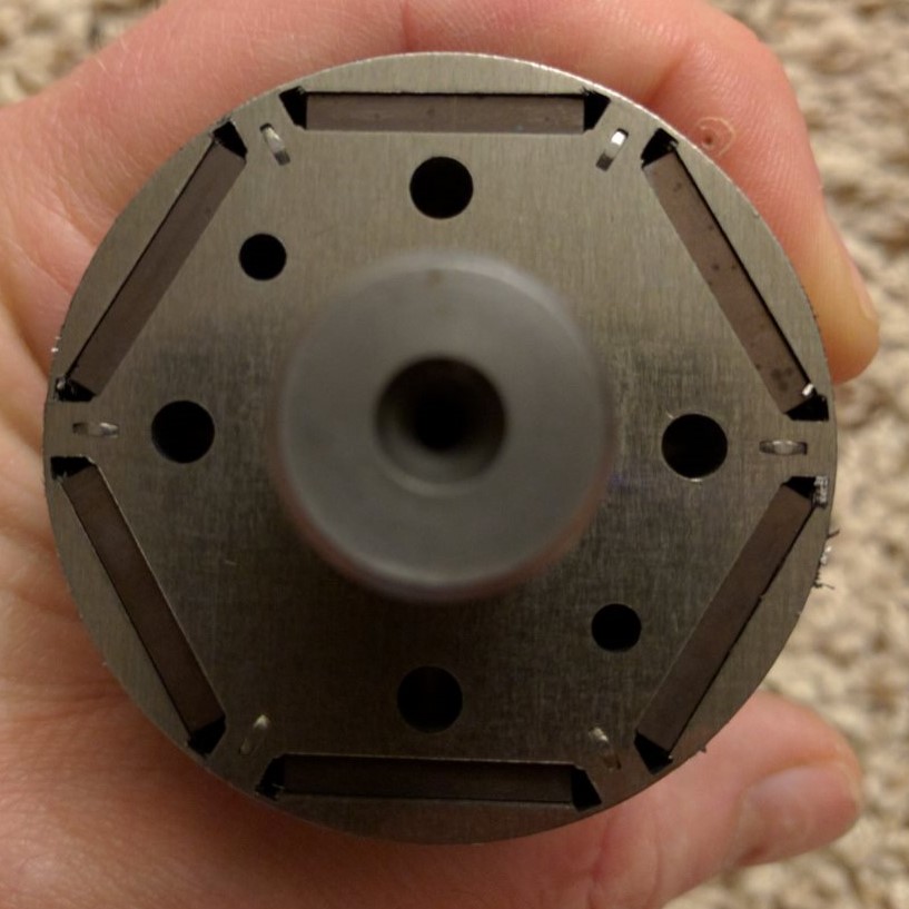 Example of IPM motor30
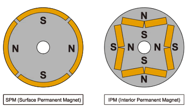 Difference between an IPM motor and an SPM motor.
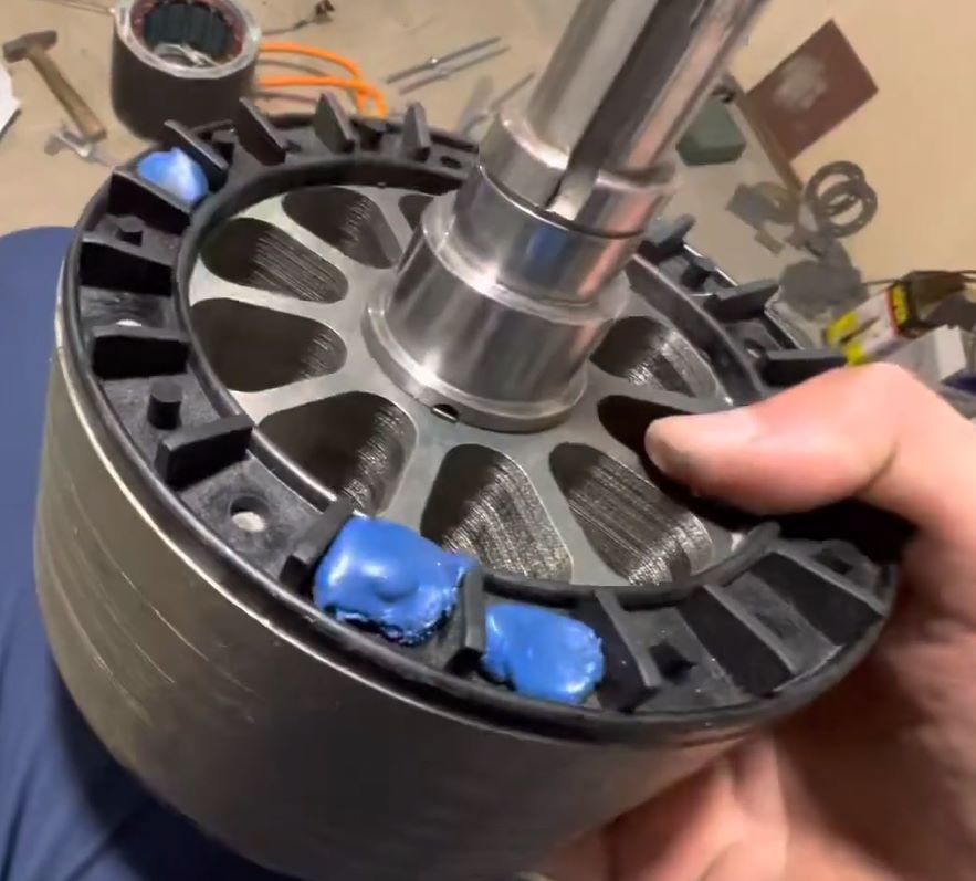 IPM motor |
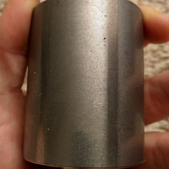 IPM motor |
IPM motors are salient pole motors. This means that the rotor of these motors is made up of laminations as can be seen in the image above. This lamination allows a reluctance torque to be generated. This means that in addition to the torque generated by the magnets, a torque generated by the magnetic field in the laminations is added.
The total torque is the combination of reluctance torque and “magnet alignment” torque.
In addition, this type of motor allows for a smaller distance between the rotor and the stator (air gap) than SPM motors, which helps to increase the flux and reluctance torque.
These motors have been developed since the 1970s, but due to their complex control because of the non-linearity between torque and current, they have had a slow evolution. Today it’s already possible to have low-cost chips that are capable of processing the signals that these motors need, which has increased their use.
It should also be noted that in these motors it’s possible to concentrate the magnetic flux. This is achieved through the use of V-shaped magnets.
These motors are also less prone to demagnetization than SPM motors.
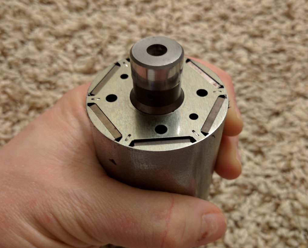 IPM motor |
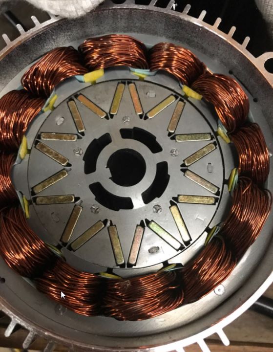 IPM motor with V-shaped magnets |
ME1616
The organization gave us the following datasheet regarding the motor of this edition:
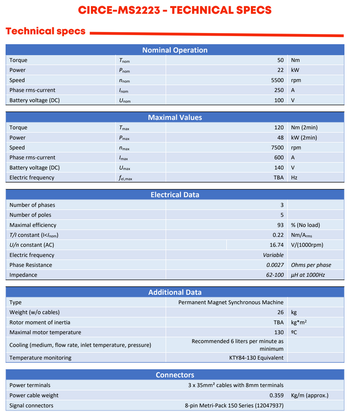 ME1616 datasheet
With these specifications we can conclude that within the motor categorization, it’s a permanent magnet motor. As we can see in the image and in the data sheet, it’s a three-phase motor (it has 3 cables for power), alternating current (AC), synchronous and permanent magnet motor, as in previous editions.
We can also see that as in any electrical machine, we have maximum values and nominal values. This indicates that during a certain period of time we can squeeze the maximum capacities of the motor, but doing so continuously would cause breakdown or problems in it. Normally these values are specified through S1 (Continuous duty: the motor works at constant load for enough time to reach temperature equilibrium) and S2 (Short-time-duty: the motor works at constant load, but not long enough to reach temperature equilibrium, and rest periods are long enough for the motor to reach ambient temperature).
After searching the internet for motors of this type, we managed to find the manufacturer, in this case Motenergy. It is the ME1616 model: (www.motenergy.com/mepmwaco.html)
I mailed the company to check if I could get more information about this motor. I got the following files:
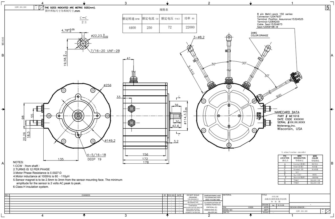 ME1616 drawings
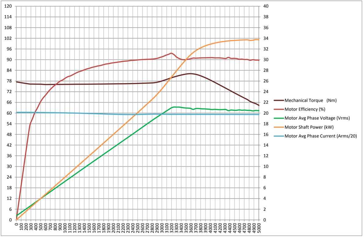 ME1616 power graph
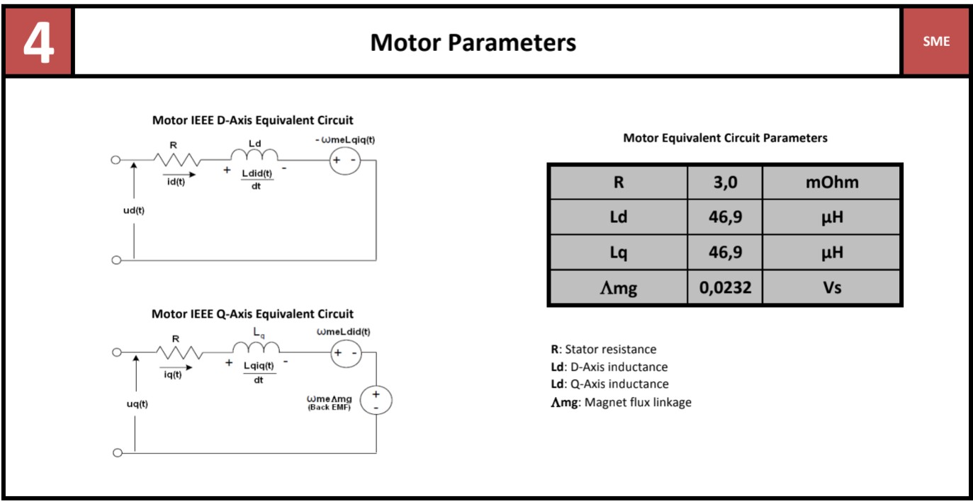 ME1616 data
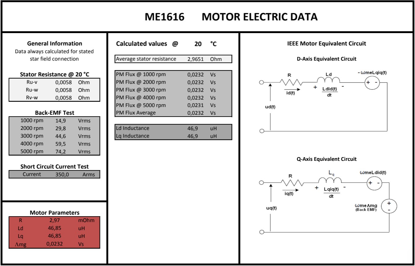 ME1616 data
ME1616 Internals31
Below are images of the internal construction of this motor32 33:
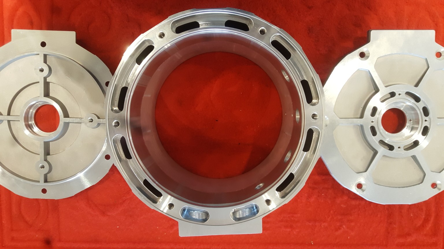 ME1616 internals
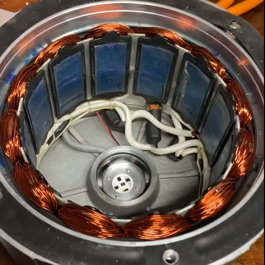 ME1616 stator |
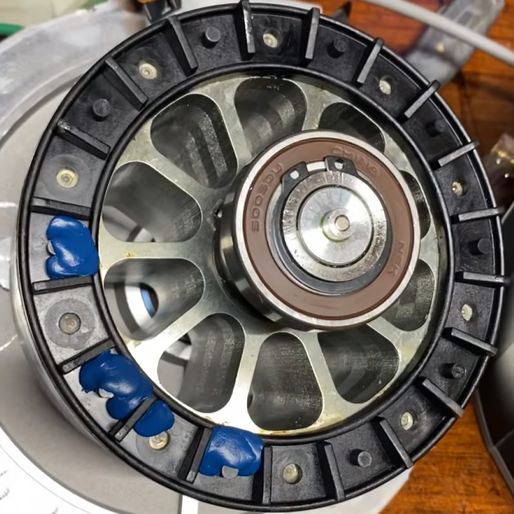 ME1616 rotor |
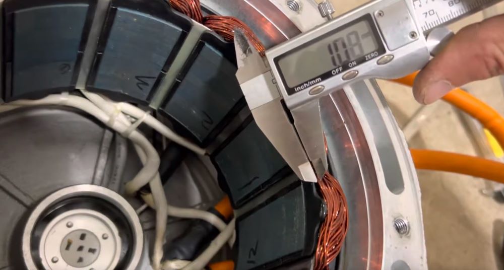 ME1616 coils |
ME1616 rotor |
Engiro34
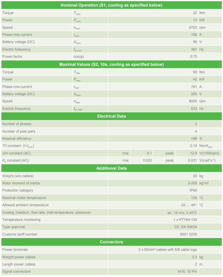 Engiro datasheet
Engiro efficiency |
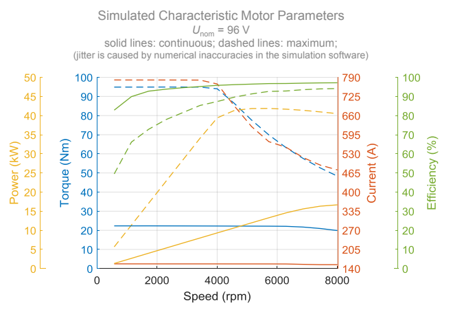 Engiro simulated |
Engiro Internals35
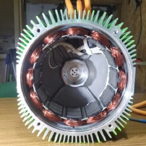 Engiro stator |
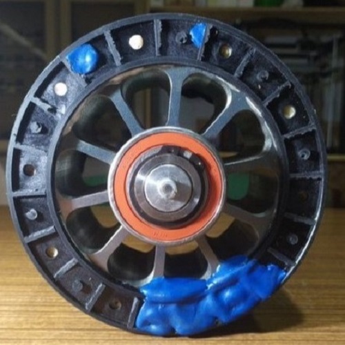 Engiro rotor |
After discovering that the motor delivered by the organization was a ME1616 from the company Motenergy, I started to search for information about the motor. I found some drawings of it where I could find a reference:
0JWT.303.269 After searching on the internet, I came across Changzhou Jintan Micro Motor Co., Ltd. (www.jintankm.com/)
This is a Chinese company that manufactures motors according to the requirements of its customers. Among its products are permanent magnet motors:
Jintan Micro Motor webpage screenshot36
There is no reference to Motenergy in the specifications and the motors they offer do not seem to have any relation to those of Motenergy, in this case the ME1616.
Searching for this company and Motenergy, I found the following post (www.diyelectriccar.com/threads/something-strange-here-about-motenergy.178849/) in which a user seems to have reached the same conclusion, and that is that the manufacturer of the motor is not Motenergy, but the Chinese company mentioned above:
Diyelectriccar forum37
Curiously, the last response in the post seems to be from the company itself (Motenergy) although we do not know if it was them or someone impersonating them:
Diyelectriccar forum37
That is, as I imagined, Motenergy designs (or subcontracts the design under its intellectual property to the company that manufactures them) and this company manufactures the motors and sends them back for distribution. On the other hand, Motenergy does not seem to have a presence in China, so the company that manufactures them distributes them under its name within the country. Even so, I still had no evidence that the manufacturer was the same one, so I continued searching on its website.
After doing some more research on the website, I found the following image (on the Chinese website, it did not appear in the English website):
Jintan Micro Motor factory
It can be clearly seen that in the image the ME1616 motors are at the bottom, so there is no doubt that it’s the manufacturer of them.
The most striking thing of all is the green motors you see on top. They seem to be Engiro motors, is it the same manufacturer?
After checking all the motors that Engiro has available, I can draw the following conclusions:
Engiro motor
Engiro motor
The image on the right is of a longer motor. Engiro uses the same render for all motors of that type regardless of size. It’s still possible to distinguish the pattern of the holes. Note also in both images the colored marking on the water inlets (red and blue).
On the other hand we can see the rotors of both motors (remember that they are completely different manufacturers, one German and the other American):
Of course all rotor designs can converge to a similar design. I understand that there is an optimal design or shape that all the studies have been able to reach and that the state of the art is in optimizing small details such as position of the magnets, distance, size, etc.
As we can see in this report: www.energy.gov/sites/default/files/2022-02/Neodymium Magnets Supply Chain Fact Sheet Final.pdf
“Rare earth permanent magnets are a critical technology for the clean energy transition and electrified transport revolution. The global supply chain for rare earth metals and magnets is almost completely dominated by China, which controlled 58% of rare earth mining and 92% of magnet manufacturing in 2020. The United States produces only 15% of the global supply of raw materials for these magnets, and while the nation has several nascent downstream processing and manufacturing efforts, current domestic production is limited.”38
Rare earth process38
In the USA there is mining and extraction of rare earths but not their processing or the manufacturing of permanent magnets as such.
www.bis.doc.gov/index.php/documents/section-232-investigations/3141-report-1/file
“China is the only country with operations in all steps of the NdFeB magnet value chain, including upstream (mining, carbonates production, and separation to oxides) and downstream (metal refining, alloy production, and final magnet production) markets. All other countries maintain operations in only some steps of the upstream or downstream magnet value chain”39
Perhaps this may be the main reason why all these manufacturers have their production in China, since it’s difficult to export these raw magnets for manufacturing in Europe, apart from the lower production cost.
In short, companies like Engiro and Motenergy are dedicated to the development and simulation of motors using software. They use multiple software such as ANSYS, Infolytica, Matlab and FloEDF to carry out the design and finite element analysis and then send their production to China where they have the technology and resources to manufacture the electric motors.
FEA on electric motor[^engiro]
Motor Parameters
Below I will describe the important parameters or characteristics to know about a motor of this type before starting to program it.
- Number of phases: Number of electrical phases the motor uses to create a rotating magnetic field. A typical PMSM has 3 phases.
- Number of pole pairs: Number of north-south magnetic pole pairs in the rotor.
- Kt (Torque constant): Defines the relationship between the motor’s input current and the torque it produces, typically in Nm/A.
- Ke (Voltage constant): It’s the ratio between the Back-EMF generated by the motor and its speed. It’s typically expressed in V/(rad/s) or V/krpm. It describes how much voltage the rotor will generate per unit of speed.
- Rotor moment of inertia: It quantifies the rotational inertia of the rotor. Represents the “resistance” of the rotor to change its rotational speed.
- Maximum motor temperature: It specifies the maximum temperature that the motor components can safety tolerate.
- Maximum revolutions: It specifies the highest rotational speed the motor can achieve.
- Continuous power: The amount of power the motor can deliver over a extended period of time without overheating.
- Peak power: Maximum instantaneous power the motor can output (typically a few seconds).
- Constant torque (rated torque): The amount of torque the motor can generate without overheating.
- Maximum torque: Highest torque the motor can generate in Nm.
These are just some of the general data needed. As we will see later, each inverter needs different data or some are calculated by the inverter, so for now these parameters will be enough.
IPMSM Characteristics
There are differences between IPM and SPM motors. These differences are not only physical, but are also reflected in the control. The algorithms used for the control of SPM motors (simpler) are valid for IPM motors, but they are not capable of obtaining their maximum performance. Therefore, we will check whether the inverter supports IPM motors. The fact that an inverter does not support IPM motors does not mean that it cannot work well with them, we are simply talking about the fact that it does not have algorithms for the MTPA, for example.
Inverter
Introduction
Let’s start, from my point of view, with the most opaque and complex part of making an electric motorcycle. In an electric motorcycle or vehicle we have a battery that stores energy. Batteries are direct current (DC) power sources. As we mentioned before, the motor that the organization has given us is a three-phase alternating current motor. This is where the inverter comes into play, it’s the element in charge of converting the direct current from the batteries into alternating current for the motor. It also works in the opposite direction, that is, it’s capable of converting the alternating energy generated by a motor during braking into direct current to charge the battery.
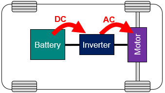
The inverter is also responsible of managing the entire motor. This means the accelerator, brake, power maps, etc. There are more complex systems in which all management is done in an external unit, but in a “simple” system like the one we use, all this management is done by the inverter itself.
When I joined the team, I had absolutely no idea about all this. I found that the inverter proposed by the organization (they had some kind of sponsorship or agreement with them) was a Sevcon Gen4.
Basic Concepts
To select the inverter that best suits our application, we must know the basic concepts and what we should look for when making the decision.
Some of the features are described below:
- Input voltage: We can say that when talking about electric vehicles, there are different voltage ranges depending on the application.
| Vehicle type | Voltage range (V) |
| Small vehicles | 12V, 24V, 36V, 48V |
| Medium vehicles | 96V |
| Larger vehicles | 300V, 400V |
| Larger vehicles | 800V |
We need to look for inverters in the range of approximately 96V. Some of the applications for this type of inverters are industrial machinery such as forklifts, platforms or carts.
Nowadays, the market tends to use high voltage in most applications. The advantages of using high voltage is that to obtain the same power, you reduce the current used. This means that the amount of conductor and semiconductor material (wires, transistors, etc.) is less, reducing costs and replacing it with insulating material (when working with higher voltage, we must use better insulation to avoid arcs). In addition to this material being cheaper, high voltage reduces the amount of heat produced by the current flow.
The negative side of high voltage is the danger it poses to people. Probably that’s the main reason why the MotoStudent regulations limit it to 126V. It is still a safe voltage for people to use if they make a mistake.
This greatly reduces the number of inverters on the market that may be suitable for our application. Furthermore, the competitive market is completely focused on high voltage, so there will not be any inverters for that direct application.
- Peak phase current: This is the maximum output current generated by the inverter. We need it to be above the maximum current supported by the motor, in this case for the acceleration test. It does not need to be much higher either, since we will not use it. On the other hand, normally the higher the supported current, the lower the switching frequency the inverter can produce, so we need a balance between both.
- Output frequency: As we will see later, this is the frequency at which the transistors switch. The higher the frequency supported, the better the output wave will be, but the hotter it will get. Some inverters allow you to configure this value.
- Encoder: The motor delivered by the organization has a sin/cos type encoder so the inverter must support this type of encoders.
- IPM support: As we have mentioned before, to get the most out of an IPM motor we need the inverter to have the necessary algorithms.
- Communication interface: This is the communication interface with the inverter. It’s used to connect it to a PC and to be able to program and monitor the inverter. They are usually CAN or UART interfaces.
- Software: Software and documentation are an important part that makes the difference between one inverter and another. Good software will help us to correctly monitor the changes we make. The more complex it is and the more parameters it allows us to modify, the better the adjustment will be, but it will also make programming more complex.
With all this clear, we can begin the search for a suitable inverter for our application.
Inverter Comparison
Let’s try to analyze some of the brands and models of inverters available on the market. There are probably more or new developments, but I will try to mention all the ones that could fit our application.
The selection of the inverter is probably the most important point of the entire prototype. Of course, without an appropriate battery (due to its capacity or because it does not provide the expected current), or a chassis that does not break, we are not going anywhere, but the inverter is that element that makes the difference, especially in a racing prototype.
To do this, I carried out an analysis of all the inverters that were on the market (or that I could find) and that met the requirements we were looking for. These requirements were mainly:
- The maximum voltage of the battery (limited by the organization) is 126 V, so the inverter had to be close to that range. To clarify, we can mount a higher voltage inverter, but normally when increasing the voltage the current they support decreases and we must remember that P = V*I so we are not interested in working at low voltage in these inverters. Also, the high voltage inverters have a higher minimum working voltage so we must avoid to be working at the minimum voltage limit.
- Sin/cos encoder support: Because the motor is delivered by the organization and we cannot modify it, the inverter we use must support a sin/cos encoder.
- IPM motor support: Although I will analyze it in detail later, it was recommended that the inverter support IPM motors. Actually any PMAC inverter should support them, but we wanted it to have the MTPA (Maximum Torque Per Ampere) and field weakening algorithms.
- Number of parameters to be adjusted: We need an inverter that allows us to adjust, within a certain limit, the largest number of parameters possible. This will make the process more complex but will make a difference if we manage to adjust them correctly.
With a clear idea of what we are looking for, we will move on to analyze the different inverters.
High Voltage Inverters
Some brands that have high voltage inverters found were:
- Scott Drive (http://scottdrive.co.nz/)
- Cascadia (www.cascadiamotion.com/)
- UniTek (www.unitek-industrie-elektronik.de/)
- DTI (www.drivetraininnovation.com/)
- WEG (www.weg.net/catalog/weg/BR/en/Industrial-Automation/Drives/Electric-Mobility/c/BR_WDC_IA_DRV_ET)
All of them have inverters that work at a voltage higher than 130V, so they are not useful for our application, in which we are limited to that voltage by regulation. I should also mention that many of the brands mentioned below have high voltage models.
Next we will analyze those that may be valid.
Curtis 1238 SE40
Tested: NO
Hardware
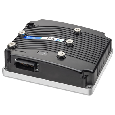 Curtis 1238 SE
| Specification | Value |
| Input voltage | 72-96V |
| Maximum input voltage | 120V |
| Minimum input voltage | 50,4V |
| Peak phase current | 900A (2 min) |
| Continuous phase current | 305A |
| Maximum controller output frequency | 450 Hz |
| Sin/cos encoder support | Yes |
| IPM motor support | ¿Yes? |
At first, this inverter caught my attention considerably. It has a peak current of 900A for 2 minutes. It is important to note that 2 minutes is approximately the time our prototype takes to complete a lap on the Motorland circuit, so for us, this current would not be considered a peak. However, as we will see later, this current is excessive for our needs since the main limitation is the motor. Still, it could be useful during acceleration testing, where the throttle is held at full position for only a few seconds and the peak amps could be beneficial.
It’s worth mentioning that this inverter is compatible with both ACIM and PMAC motors, although its approach is somewhat different for the second one. Curtis offers a list of 127 pre-parameterized or characterized motors, which is advantageous if the motor is on the list, as is our case with the ME1616. However, this pre-configuration has a disadvantage: the lack of flexibility to adjust these parameters. Since our application is special (competition), we don’t know if the characterization performed is aimed at maximizing motor performance or simply offering good performance without squeezing the most out of its features. This was the main reason why we decided not to use this inverter along with its high price (over 3000 €).
Regarding IPM motor support, I didn’t find any evidence in the documentation I had access to that this inverter properly supports IPM motors or implements MTPA. However, on the Curtis’ website it’s mentioned that they offer dynamometer services, and the following is detailed:
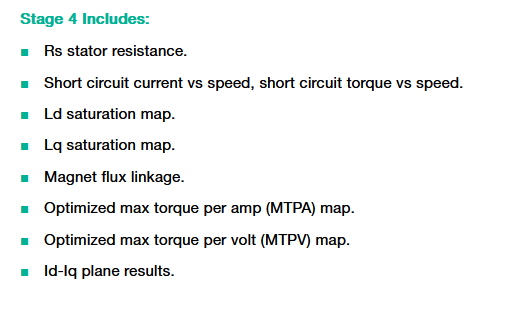
So I assume that within the characterized motors they use all this information by applying the MTPA algorithm, although I have not been able to verify this.
From what can be seen in the documentation, it looks like it has auto-tune. It should be noted that this type of process is valid for making an initial setup, but, in general, manual adjustment is necessary after the process to optimize certain parameters.
It’s also worth noting that it has support for VCL (Vehicle Control Language) through the WinVCL software, although I cannot say much more about it because I have not tested it.
On the other hand, I would like to comment that after a brief conversation with an expert who had programmed this type of inverter, he told me that Curtis has a fairly good control in speed mode, but in this case it does not apply to us since we use the inverters in torque mode for this application.
Software
To connect the inverter we need to have the interface, which in this case is USB-Serial (probably UART). It is a expensive interface, between 300 € and 400 €.
 Curtis PC USB-Serie interface
For parameterization we have the software 1314 PC Programming Station, programmed in Delphi. I have not been able to test it personally but from the images I have been able to obtain it looks like a simple software, with everything organized.
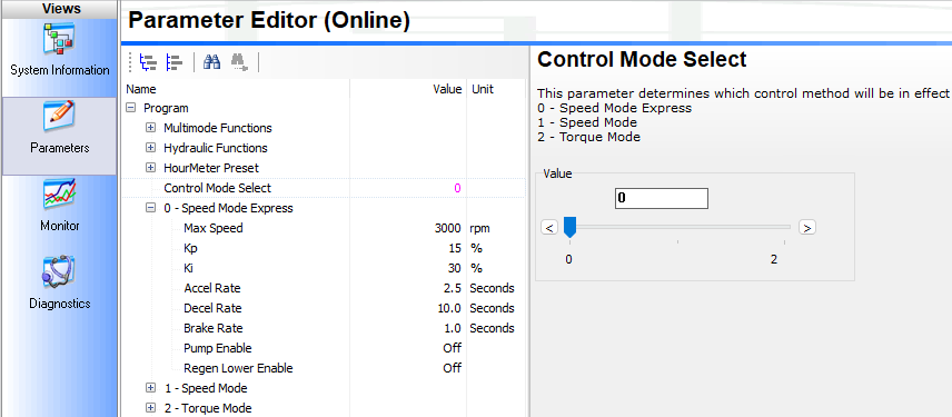
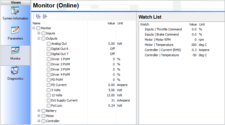
As for Curtis’ documentation, although it’s somewhat difficult to find (it’s not on their official website), it’s true that it’s quite complete and organized, detailing the steps necessary to start up the inverter.
Regarding the software, it’s worth noting that they are developing a new generation of inverters (F series) and the software seems much more complete, especially in the monitoring part, which is what I have missed the most in other inverters.
EmDrive 50041
Tested: NO
EMSISO d.o.o is a Slovak company engaged in electronics research and development. It offers a range of inverters for both high and low voltage. In this case I will analyze the emDrive500, which is the model that best suits our application.
Hardware
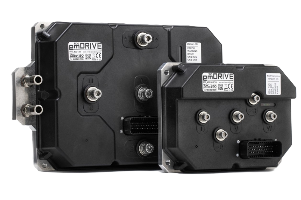 EmDrive 500
| Specification | Value |
| Input voltage | 30-120V |
| Maximum input voltage | 120V |
| Minimum input voltage | 30V |
| Peak phase current | 800A (1 min) |
| Continuous phase current | 500A |
| Switching frequency | 16 kHz |
| Sin/cos encoder support | Yes |
| IPM motor support | Yes |
At first, this inverter gave me a very good feeling. To start with, it has liquid cooling as standard, which allows it to support a high continuous current (500A). Another interesting feature was its maximum current of 800A and its maximum voltage of 120V.
After studying the documentation, another positive point is the implementation of an MTPA algorithm for IPM motors as well as field-weakening. In addition, the documentation details the models used for torque control, MTPA and field-weakening, which helps a lot to understand what we are dealing with when parameterizing it. From my point of view, this is one of the problems that other inverters such as Sevcon have, the “opacity” of the model used for control, which makes you work blindly.
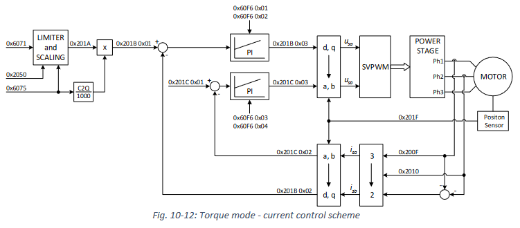 Torque control model of emDrive500
If these algorithms are the ones that are actually implemented in the inverter, it would allow us to represent it in some software such as Matlab and perform simulations to optimize the parameterization of them.
However, a couple of negative points that I found were that they didn’t have regenerative braking implemented. Also, they used the same input connection for the sin/cos encoder and for the power selection (eco, normal, sport).
Software
To connect the inverter we need the proprietary USB-CAN interface.
 USB to CAN
As for the software, we have a program (considering that it has not been fully developed) programmed in C# or Visual .NET. It has monitoring tools, although I have not been able to test it because it requires a license for its use and I didn’t have an inverter to connect to.
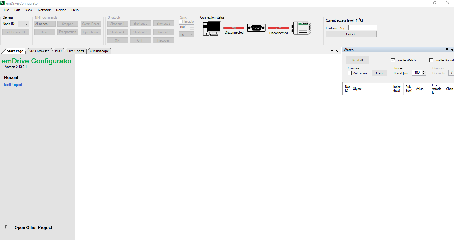 Initial view of the software
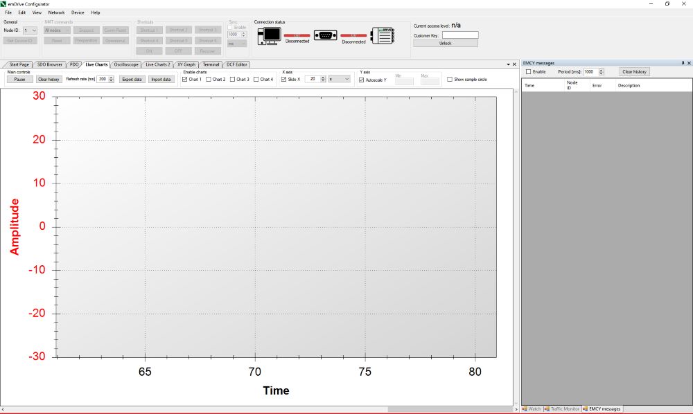 Monitoring screen
One of the interesting elements of this inverter is that it has implemented the MTPA algorithm for IPM motors. Unlike Sevcon, which uses tables to define the Iq and Id values based on revolutions, torque and voltage, this implementation is done through a second degree polynomial:
 MTPA polynom
I find it an interesting approach and at first easy to parameterize, although I do not know the quality of the result it generates.
In my opinion, they have excellent documentation, detailing implementations of different controller algorithms as mentioned above and with a step-by-step description of the implementation of the controller with examples. It’s also worth noting that it has self-alignment for the encoder.
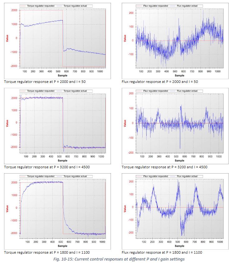 PI tuning example in emDrive documentation
However, there are several points that led me not to choose this inverter. Reading the documentation carefully, it’s clear that this is an unfinished development. For example, as mentioned above, they have not yet implemented regenerative braking and after contacting them they told me that they did not plan to implement it in this generation of inverters. It should still be said that the software seems to be updated periodically, what I do not know is whether with new features or bug fixes. Also, when I contacted them to ask for the price and delivery time for a unit, they required the purchase of (I think I remember) two units as a minimum and the delivery times were very long because they didn’t have products in stock and had to wait to have enough orders to manufacture units.
I have also been following the documentation updates but unfortunately they have not updated it for a couple of years (to date), so it seems that development is a bit stagnant. After speaking with a team that had used it this year, they told me that they had not managed to adjust the field-weakening correctly. Of course we don’t know if it’s really a problem with the inverter or the team’s skills when setting it up.
www.emdrive-mobility.com/portfolio/emdrive-500/
Kelly KLS-XXXX42
Tested: NO
Hardware
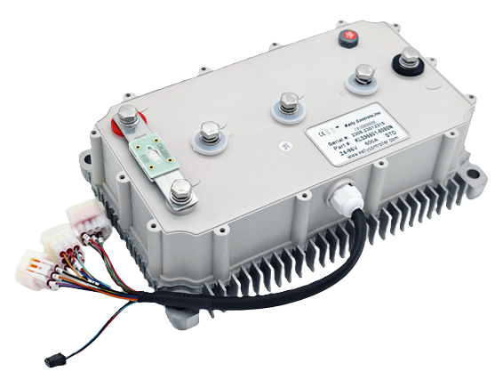 |
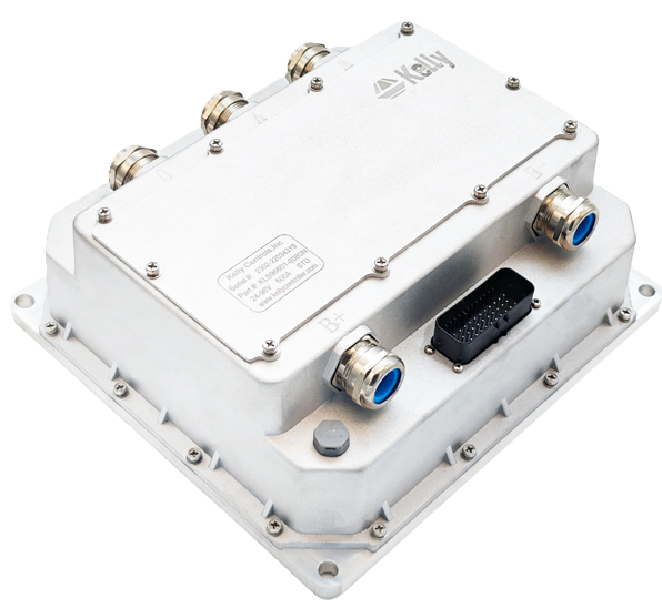 |
| Specification | Value |
| Input voltage | 24-96V |
| Maximum input voltage | 115V |
| Minimum input voltage | 24V |
| Peak phase current | 400 - 1100A (1 min) |
| Continuous phase current | 240 - 600A |
| Sin/cos encoder support | Yes |
| IPM motor support | No |
We have an inverter developed and manufactured in China. At the time of choosing the inverter for the prototype, the available offering was much more limited compared to today. In this context, Kelly’s KLS series offers inverters that operate up to 120V and 1100A. At the time of making the decision, I remember that the most powerful inverter available was 96V and approximately 450A, although I am not sure.
It’s clear that there have been improvements in the hardware, two factors influenced the decision not to select this inverter. Firstly, the documentation and datasheets do not mention support for IPM motors (e.g. the MTPA algorithm) at any point. Secondly, the configuration capacity of this inverter is limited, as can be seen below.
It is important to note in its favor that it has an encoder self-alignment function, although I cannot comment on the quality as I have not tested it.
Software
To connect to the inverter, we need a USB RS232 interface. According to the documentation, it seems to be a generic interface.
As you can see in this screenshot, these are all the parameters that the inverter allows you to configure. This means that we don’t have too much freedom of configuration, and in an application like the one we are looking for, I consider this to be something fundamental.
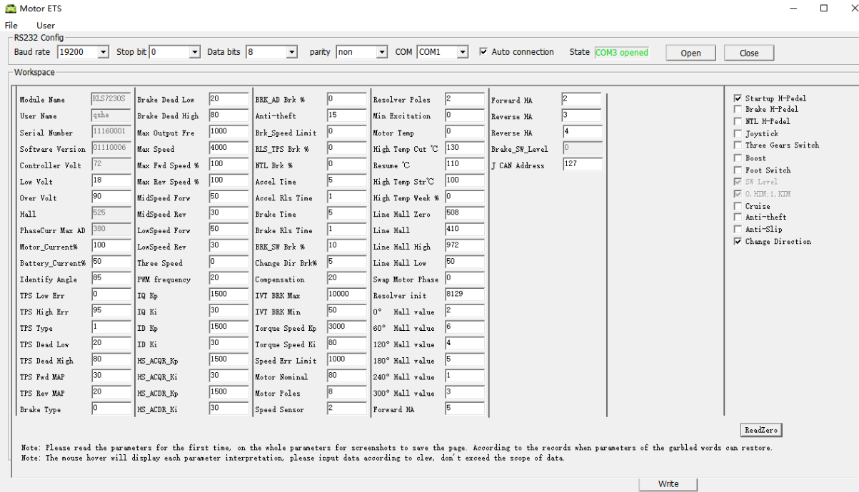 Parameter configuration
As for monitoring, we have a fairly simple interface that only allows monitoring of all data in real time, but it does not seem that the results can be saved or exported for later analysis.
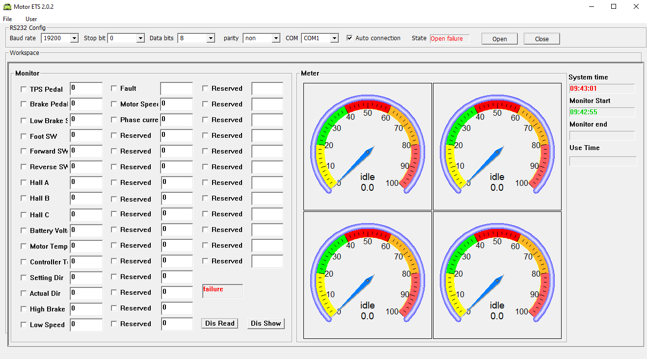 Monitoring screen
The lack of support for IPM motors, the poor quality of the software and the limited configuration capacity available on this inverter were the reasons why I decided not to go with it, and at the time of the decision, the most powerful model did not offer any notable features compared to other inverters.
Zapi BLE543
Tested: NO
Hardware
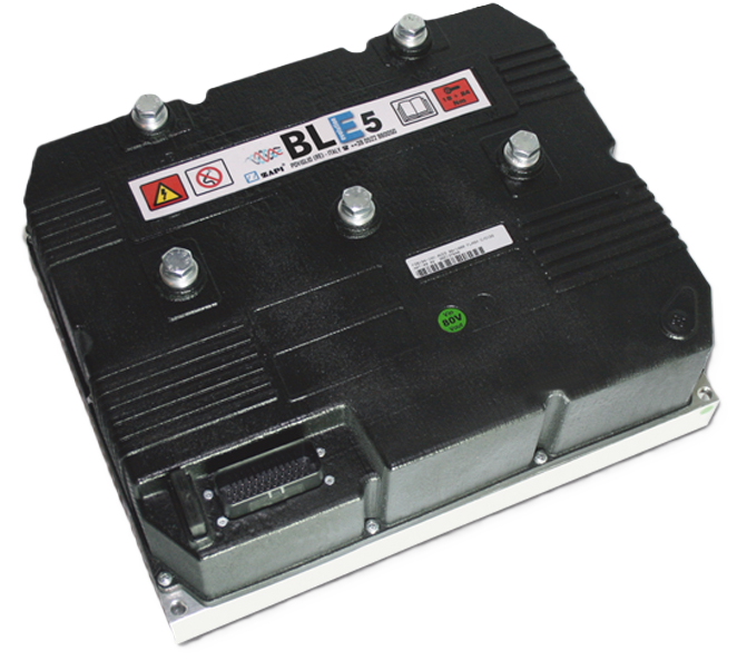 Zapi BLE5
| Specification | Value |
| Input voltage | 96 - 120V |
| Maximum input voltage | 120V |
| Minimum input voltage | - |
| Peak phase current | 750A (2 min) |
| Continuous phase current | - |
| Switching frequency | 8 kHz |
| Sin/cos encoder support | Yes |
| IPM motor support | No |
Zapi is one of the brands I have known for a long time due to its widespread use in forklifts. After analyzing the data sheets, I think the right model for this type of motors is the BLE5, although there is not enough public documentation to be sure (the other option is the ACE5). From what I have been able to see, the ACE5 does not support sin/cos encoder input, and in theory, the BLE5 is prepared for synchronous motors.
After reviewing the documentation, I could not find support for IPM motors. In addition, it didn’t allow the configuration of too many parameters for motor torque control, being limited mainly to handling (accelerator, braking, etc.). Additionally, based on the experience of the previous year, a team with which we shared the box used this inverter and didn’t obtain good results.
It’s worth mentioning that the inverter has autotune to characterize the motor, but as I mentioned before, this is only an initial step for its configuration.
Software
The connection interface to the inverter is done through a CAN port. To connect, we can use different interfaces such as IXXAT, KVASER, VECTOR, among others, all of them with a high price. In our case, since we had an IXXAT interface, this was not a problem.
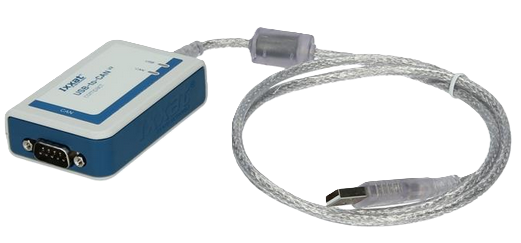 IXXAT USB to CAN
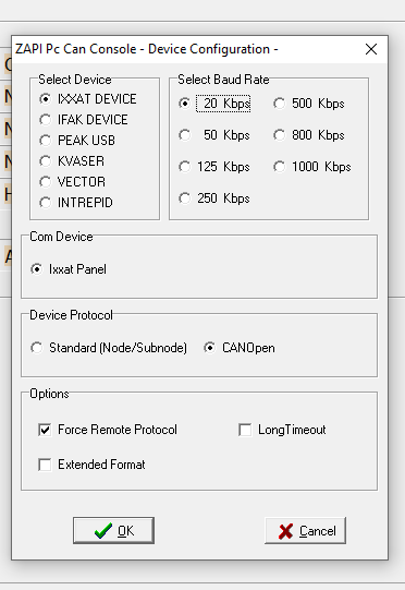 Supported CAN interfaces
The software is ZAPI PC Can Console. This is a simple software that has been in use for many years. It mainly has two main screens: one for parameter adjustment (including motor configuration, drivability, etc.) and another for monitoring the CAN signals.
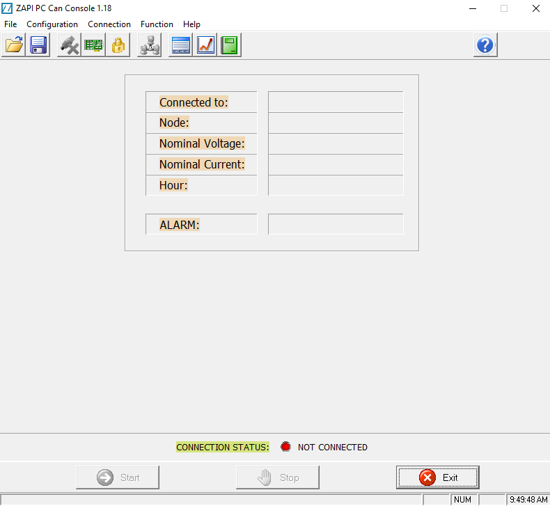 Main screen
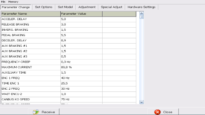 Parameter configuration
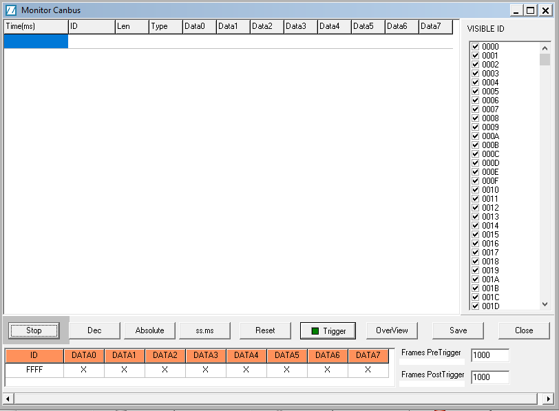 CAN monitoring
Due to the limited possibility of configuring the control and adjustment parameters of the motor, the lack of support for IPM motors and the negative experience of another team in the previous edition, this inverter did not offer anything different from others, so we did not take it as an option.
www.zapigroup.com/it/ac-evolution-series-inverters
DMC (SuperSigma2) IPM960T444
Tested: NO
Hardware
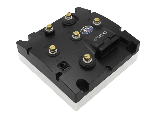 DMC IPM960T4
| Specification | Value |
| Input voltage | 96V |
| Maximum input voltage | 144V |
| Minimum input voltage | 14V |
| Peak phase current | 600A (2 min) and peak of 1110A |
| Continuous phase current | 300A |
| Switching frequency | 16 kHz |
| Sin/cos encoder support | Yes |
| IPM motor support | Yes |
We are looking at a controller from the German brand DMC. According to its documentation, it has support for IPM motors with sin/cos encoders.
I started to get interested when I recognized it among the kits that the company ENGIRO sells for its motors. This company produces IPM motors, so if they had partnered with DMC, they should support these motors in order to obtain their maximum performance.
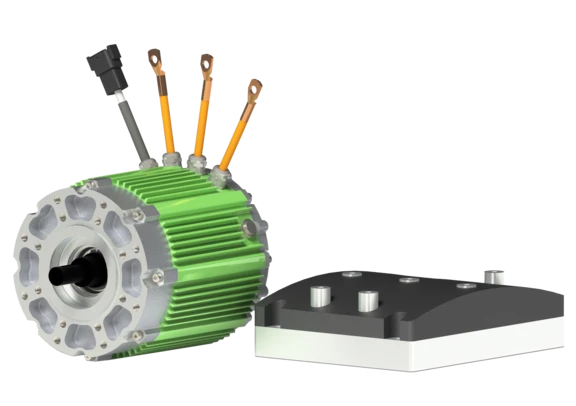 Motor-inverter assembly sold by the company ENGIRO
The documentation and datasheets state that they support IPM, but I couldn’t find any more information as there are no public manuals. After analyzing the software and configuration files, I was able to find the following:
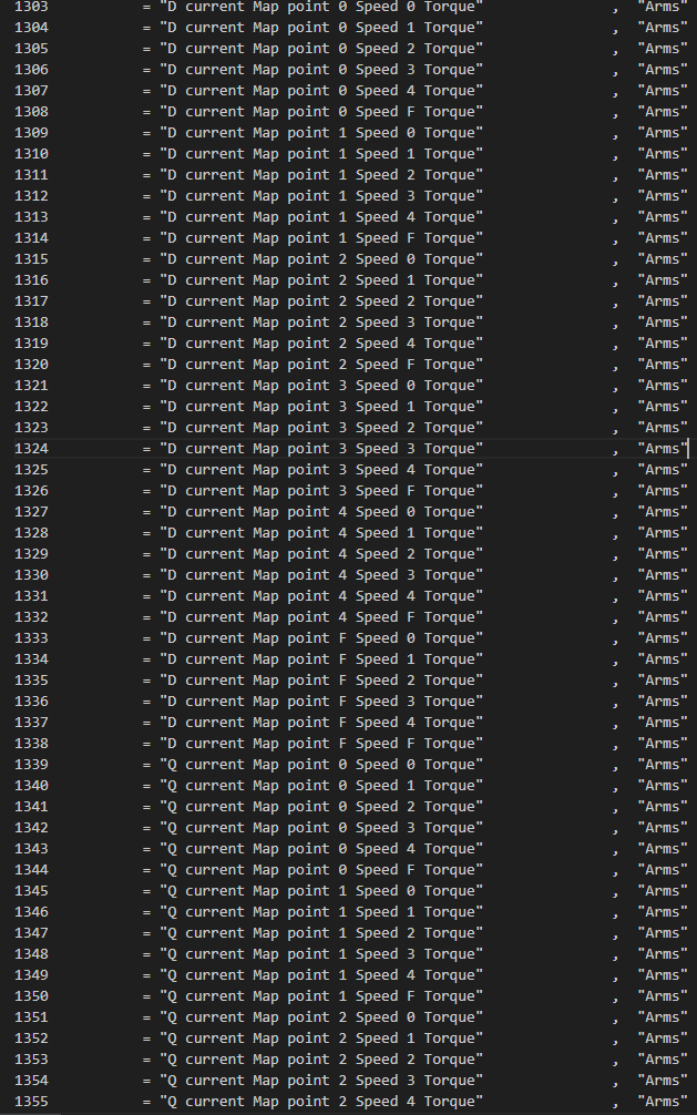 DataDictionary file parameters
It seems that this inverter has support for IPM motors. It does something similar to Sevcon, having hardcoded tables with the Id and Iq values to apply.
As we will see later, Sevcon has two tables, one for Id and one for Iq, with the motor speed on one axis and the torque on the other axis, 14x14 in size. In addition, there are 9 versions of these two tables depending on the voltage that the inverter handles.
In this inverter, from what I have been able to see (I have not been able to test it), there are two tables, one for Id and one for Iq, both 6x6 with the speed and torque applied to the motor on each of the axes. I don’t know if it also has some kind of variation based on the battery voltage.
With this, I can come to the conclusion that, unlike Sevcon as we will see later, this inverter allows you to modify the value of the tables for Id and Iq. This give us the chance to perform MTPA and field-weakening control on IPM motors.
Software
To connect to the inverter we need a USB to CAN interface called CANopen Calibrator. This is a proprietary interface that they sell.
 DMC CAN interface
The program used is DMC Configurator. At the graphical interface level, everything is quite organized and clear. We have a menu on the left that allows us to access the configuration of the inverter parameters, CAN configuration and signal monitoring, among other things.
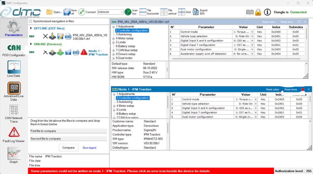 Overview of inverter parameters
It allows us to select the TPDOs we want to monitor and view them graphically in the software itself, a very positive point that makes programming the inverter easier. This is an advantage over Sevcon, where you need to open the file in Excel or another software to be able to graph it. It also has another window to show the live data, but I have not been able to test it, so I have no evidence of what is shown in it.
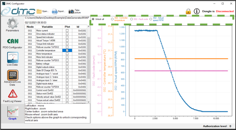 Monitoring screen
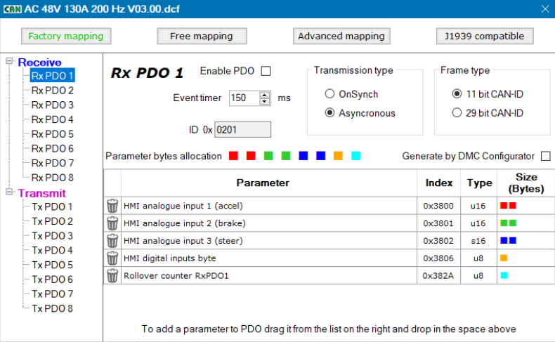 TPDOs and RPDOs configuration
As I mentioned earlier, when making the decision for an inverter, either I didn’t have enough information or the support for IPM motors wasn’t fully developed. After further analysis, it seems to me a controller that could be a good choice as long as we have the inductance values Ld and Lq, since it seems possible to edit these values and generate our own tables, unlike Sevcon as we will see later.
MGM Compro HBCi 32012045
Tested: NO
Hardware
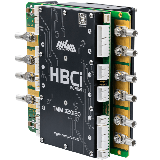 MGM-Compro HBCi 320120
| Specification | Value |
| Input voltage | 63 - 120V |
| Maximum input voltage | 120V |
| Minimum input voltage | 63V |
| Peak phase current | 600A |
| Continuous phase current | 320A |
| Switching frequency | - |
| Sin/cos encoder support | Yes |
| IPM motor support | - |
At the time of making the decision of which inverter to use, there was no such powerful model, so we ruled it out. After analyzing this model, it seems quite interesting in terms of the current it supports and the voltage at which it works. Even so, I don’t have enough information to evaluate it correctly. The website indicates that it has 69 adjustable parameters. If these parameters cover the entire inverter, they are probably few, but again, I cannot evaluate it without having that information or knowing what they are.
On a visual level, we could say that it gives us a bittersweet feeling regarding the hardware. The inverter does not have any type of external casing or protection from the elements. This is probably due to the fact that it’s an inverter focused on aeronautics, where the development priorities have been other, such as weight.
Software
The connection is made through a proprietary interface called OPTOCOM6i, which is probably CAN or RS232.
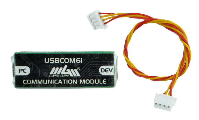 Optocom6i
The software is MGM ProTool. It is available for download on their website, but without the inverter it’s not possible to test it.
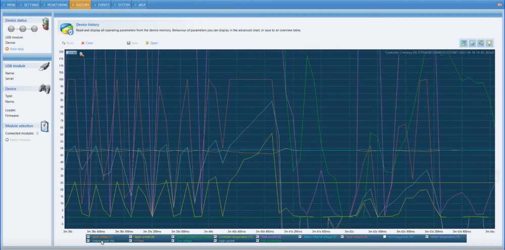 MGM Protool monitoring.
As I mentioned before, the main reason we didn’t select this inverter was the low power it supported. Also, nowhere does it specify that it supports IPM motors, so it doesn’t offer us any advantage over other inverters.
www.mgm-compro.com/brushless-motor-controllers/38-kw-motor-controllers/
Exro AS020-100V46
Tested: NO
Hardware
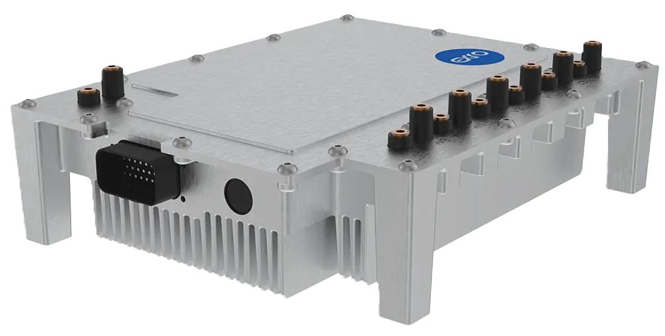 Exro AS020-100V
| Specification | Value |
| Input voltage | 36-100V |
| Maximum input voltage | 120V |
| Minimum input voltage | 36V |
| Peak phase current | 280A |
| Continuous phase current | 100A |
| Switching frequency | - kHz |
| Sin/cos encoder support | Yes |
| IPM motor support | - |
The interesting model for us was the A020-100V. Unfortunately, we cannot find much information on their website. The only thing that is known is that it works up to 120V, which would be suitable for this application. However, it has a maximum current of 250A, which is insufficient for our application, with the maximum continuous current being 100A.
It’s stated in one of the documents that it’s prepared for IPM motors, but there is no proof of this.
Software
Unknown
www.exro.com/technology/coil-driver-traction-inverter#low-voltage
Inmotion AC SuperDrive Gen6 ACS80XL47
Tested: NO
Hardware
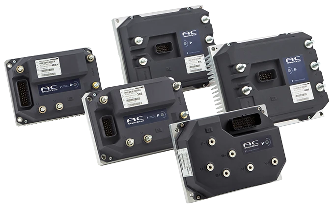 Inmotion AC SuperDrive Gen6 family
| Specification | Value |
| Input voltage | 80V |
| Maximum input voltage | - |
| Minimum input voltage | - |
| Peak phase current | 550A (2 min) |
| Continuous phase current | 250 |
| Switching frequency | 8 kHz |
| Sin/cos encoder support | Yes |
| IPM motor support | - |
Currently, two generations of products are available: ACS6 and ACS7. However, there is no evidence of the availability of the ACS7 generation. Therefore, we must focus on the ACS6 generation.
Regarding the available information, we only have a datasheet that presents the values specified in the table above. The documentation doesn’t mention details about IPM motors, and the initial features offered don’t seem to stand out significantly..
Software
There is no information available about the software used to configure it, and I have not been able to locate additional information.
https://evs-inmotion.com/en/acs-gen7-inverters
Golden motor48
Tested: NO
Hardware
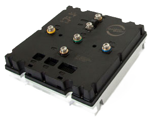 Golden motor inverter
| Specification | Value |
| Input voltage | 120V |
| Maximum input voltage | 120V |
| Minimum input voltage | Unknown |
| Peak phase current | 750A (3 min) |
| Continuous phase current | Unknown |
| Switching frequency | 8 kHz |
| Sin/cos encoder support | Yes |
| IPM motor support | Yes |
We have two series of inverters, the EZkontrol series and the VECTOR series. I have not been able to draw conclusions regarding the difference between the two as the documentation is scarce. It has autotune for parameterization of the motors but I have not found much more information on this subject.
Regarding IPM motors, I have not been able to find evidence of support for these motors. In addition, from what I have been able to analyze, it does not support sin/cos encoders, so it is completely invalid for our application.
Software
For connection to the inverter we have an interface that appears to be USB-RS232 as indicated in the electrical diagrams.
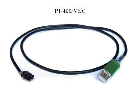 USB to RS232
We can find a very basic program in which we can adjust the parameters. After analyzing them, we can see that the list is quite short, so I assume that it does not support IPM motors either.
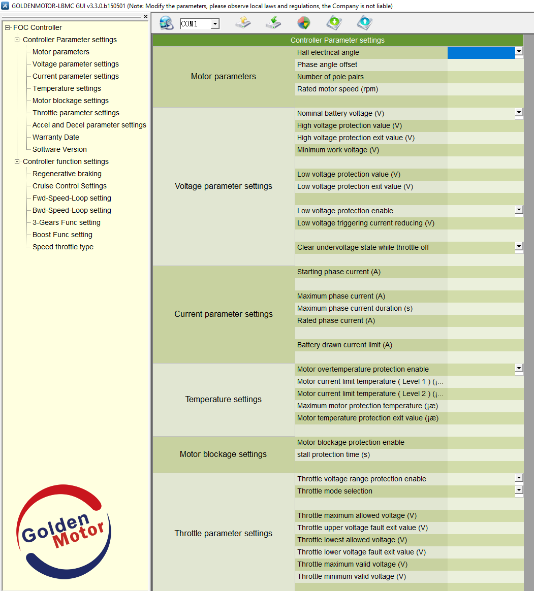
With this small configuration, without support for sin/cos encoders and without offering any substantial advantage we can say that it is ruled out.
Roboteq RGBL189649
Tested: NO
Hardware
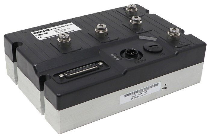 Roboteq RGBL1896
| Specification | Value |
| Input voltage | 96V |
| Maximum input voltage | 100V |
| Minimum input voltage | 40V |
| Peak phase current | 300A (30s) |
| Continuous phase current | 200A |
| Switching frequency | - |
| Sin/cos encoder support | Yes |
I have not been able to locate the RGBL1896 model on their website so I do not know if it is available. The RGBL1860 model is available but it only supports 60V which is insufficient for our application. The 96V model theoretically supports 300A peak which is also not enough for what we are looking for. However, the positive point is the number of adjustable parameters it has and the support for IPM motors as we will see below.
Software
RoboteQ has a software that looks quite good. It’s also worth noting that everything is very well documented, which makes programming the inverter easier.
On the positive side, it’s worth mentioning that it implements the MTPA algorithm for IPM motors by introducing the Ld and Lq inductances. I do not know the quality of the implemented MTPA algorithm and whether it’s possible to obtain good performance only with these values instead of lookup tables or polynom.
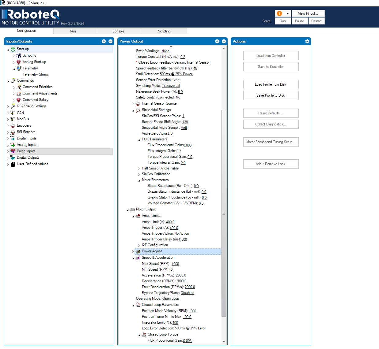 RoboteQ software
This inverter is discarded due to the low voltage and current supported, which makes it far from other inverters with superior characteristics.
www.roboteq.com/products/products-brushless-dc-motor-controllers/rgbl1860-detail
Accelerated Systems BAC800050
Tested: NO
Hardware
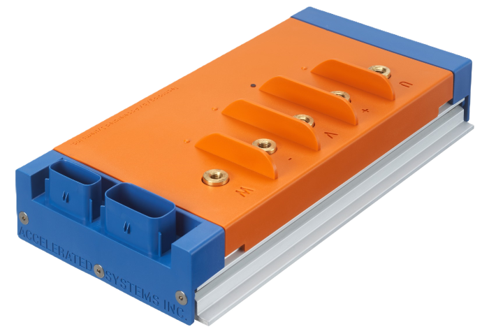 BAC8000
| Specification | Value |
| Input voltage | 36 - 72V |
| Maximum input voltage | 86V |
| Minimum input voltage | 30V |
| Peak phase current | 840A |
| Switching frequency | 10-17kHz |
| Sin/cos encoder support | Yes |
Due to its maximum voltage of 86V, it’s far from the maximum 130V that we are looking for, so it’s clearly discarded as a choice. In addition, there is not much public documentation about the software or its features in more detail.
Software
Unknown
www.acceleratedsystems.com/products/electric-motor-controllers/bac8000
Semikron SKAI 3 LV + Silicon Mobility OLEA T2225152
Tested: NO
Hardware
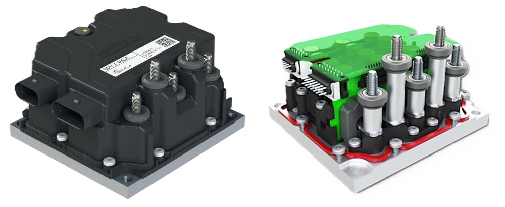
| Specification | Value |
| Input voltage | 24-120V |
| Maximum input voltage | 144V |
| Minimum input voltage | 24V |
| Peak phase current | 600A (2 min) |
| Continuous phase current | 220A |
| Switching frequency | - |
| Sin/cos encoder support | Yes |
| IPM motor support | Yes |
We have an inverter developed by Semikron with the characteristics indicated in the table above.
At first glance it seems to be a fairly compact inverter for the power it seems to support. However, after doing some research I realize that it’s only the power stage. Semikron has developed the entire power part of the inverter to allow the client to develop all the electronics and programming applied to it. In case anyone is wondering, a development of these characteristics is something very complex that would take years and a lot of knowledge to implement in an efficient way and for it to work reasonably well.
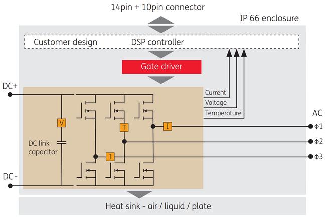 Semikron power stage
This is where Silicon Mobility comes in. The company is dedicated to developing the control part, as we can see below:
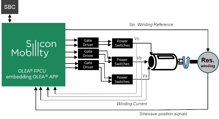 Silicon Mobility electronics
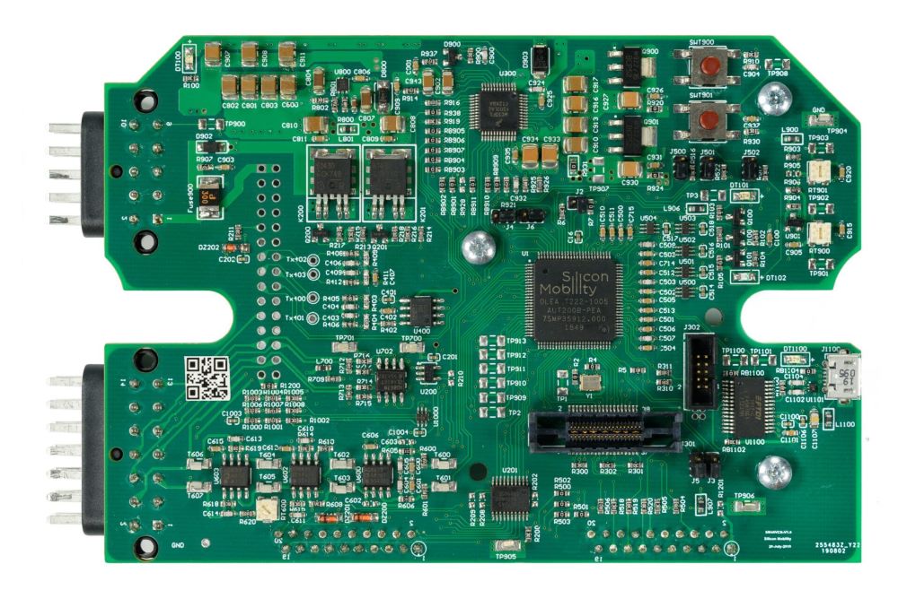
The inverter has IPM motor support through lookup tables, just like Sevcon. From my point of view, it could be a good option if you have a very deep knowledge of the subject and it could make a difference. The reality for us is that it’s a very complex environment. I don’t know the level of development by Silicon Mobility and the ease of parameterization, but apart from that complexity, the development environment is very expensive. It’s an option that draws my attention quite a bit, but realistically, with the knowledge and little time that we had available together with the budget, this option was not viable.
www.silicon-mobility.com/products/olea-app-2/olea-app-inverter-ed-2/
www.semikron-danfoss.com/products/product-lines/skai/skai-lv.html
3ShulMotors CL100053
Tested: NO
Hardware
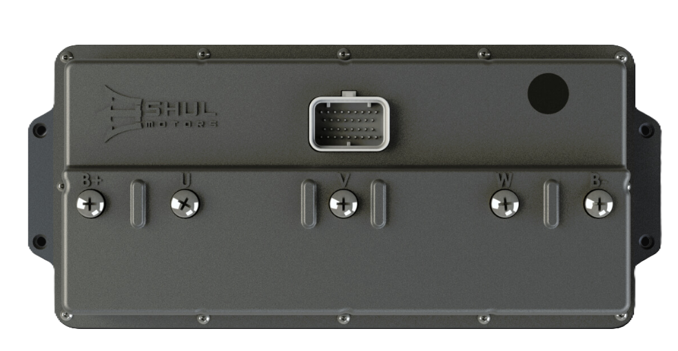 3ShulMotors CL1000
| Specification | Value |
| Input voltage | 96V |
| Maximum input voltage | 126V |
| Minimum input voltage | 36V |
| Peak phase current | 1000A (30s) |
| Continuous phase current | 500A |
| Switching frequency | - |
| Sin/cos encoder support | Yes |
It’s an inverter designed and manufactured in India. It has an STM32F4 microcontroller and uses the VESC implementation for the control system.
It has support for sin/cos encoders although I don’t know the quality of the hardware.
It’s an inverter that may be interesting to try and if the hardware is well manufactured, I think it can give interesting results.
Software
VESC is an open source system for motor control. I had only seen it implemented in small inverters so I am surprised to see this application.
It has support for field weakening and MTPA and the VESC software is quite complete.
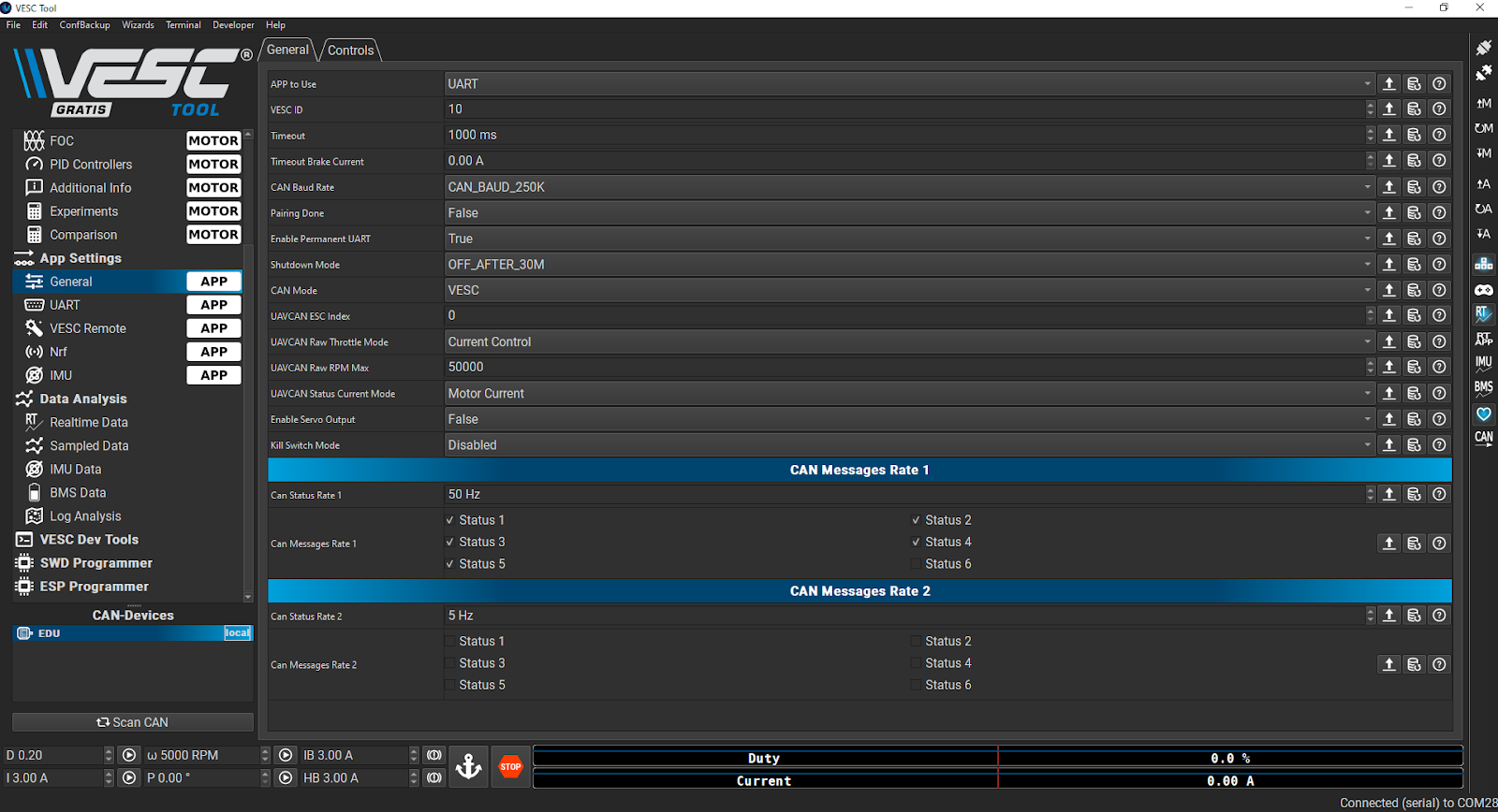 VESC software
It’s an inverter that I want to try and I think it could be an interesting option. For the IPM motor configuration, I think it automatically calculates the inductances Ld and Lq. It may not be as precise as Sevcon with the lookup tables but it can probably easily give good results.
https://3shulmotors.com/product/cl1000/
Engines Engineering54
Tested: NO
Hardware
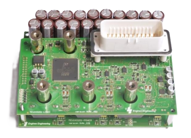
| Specification | Value |
| Input voltage | 96V |
| Maximum input voltage | 117V |
| Minimum input voltage | - |
| Peak phase current | 300A (2 min) |
| Continuous phase current | - |
| Switching frequency | - |
| Sin/cos encoder support | Yes |
| IPM motor support | Yes |
Engines Engineering is an Italian company that has been working in the motorsport world for years. There is not much information about their inverter, the only information available is the information that can be seen in the table above.
It seems to be an inverter developed by themselves. The UNIBO Motorport team uses it (they are the team’s main sponsors) but we can’t see much more.
Some features that can be observed are that it supports a current of 300A (we don’t know if continuous or peak) and that it implements algorithms for MTPA and Field weakening. Seeing that the BMS developed supports a 28S battery (117.6V peak), probably the inverter works at that maximum voltage although I can’t guarantee it.
www.enginesengineering.com/en/engines-engineering-power-train/
Dana TM4 AC-X155
Tested: YES
Hardware
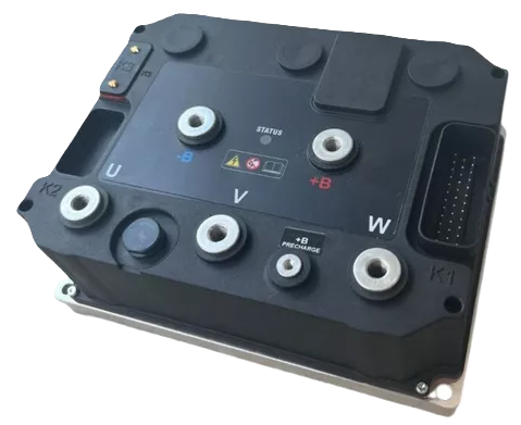 Dana TM4 AC-X1
| Specification | Value |
| Input voltage | 80-100V |
| Maximum input voltage | 130V |
| Minimum input voltage | 52V |
| Peak phase current | 750A (2 min) |
| Continuous phase current | 375A |
| Switching frequency | 9 kHz |
| Sin/cos encoder support | Si |
| IPM motor support | Unknown |
We have an inverter initially developed by the SME group company. It was later acquired by DANA under the TM4 Tautronic series. Specifically, the model that best applies to our case is the AC-X1.
This inverter has also been used by Zero Motorcycles together with Sevcon.
Almost at the end of the project we got a budget for this inverter so I was able to test it on the dyno. The advantages over the Sevcon Gen4 Size6 are its small size, ease of programming and its superiority both in maximum input voltage (130v vs 120v of the Sevcon Gen4) and its maximum current (750A compared to the 660A). On the other hand, this ease of programming prevents configuring as many parameters as the Sevcon Gen4.
It should be noted that I didn’t spend as much time on this inverter as on the Sevcon Gen4.
DANA TM4 internals
Due to a fault (short circuit at the contactor output) I had to disassemble the inverter to replace some resistors and the transistor of this output. Thanks to its modular structure (unlike Sevcon Gen4), it is possible to access all the components and replace the elements. Below are some photos of the interior:
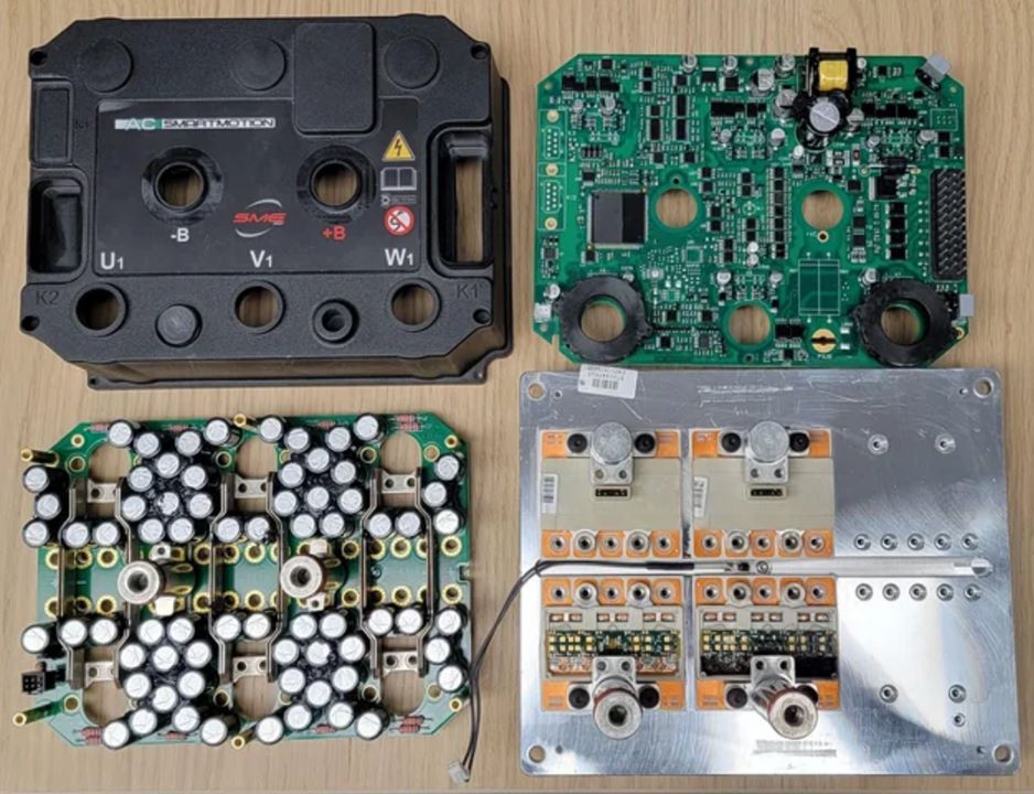 Opened inverter
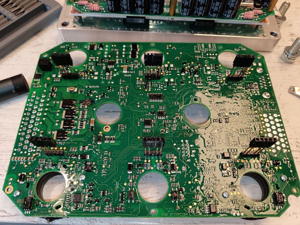 Control PCB |
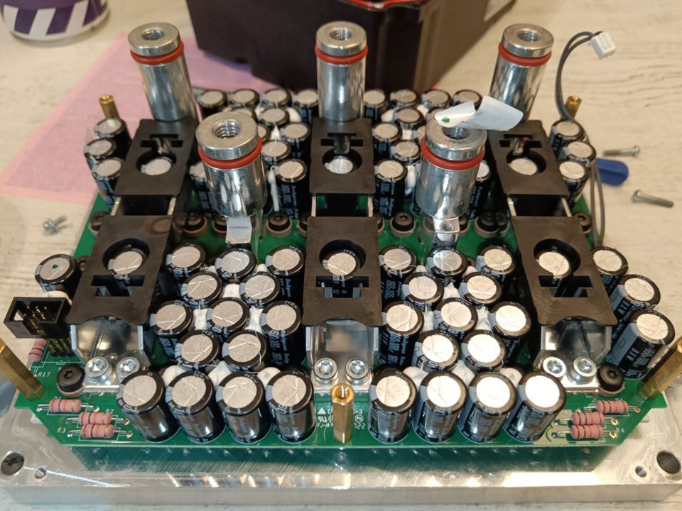 Power PCB |
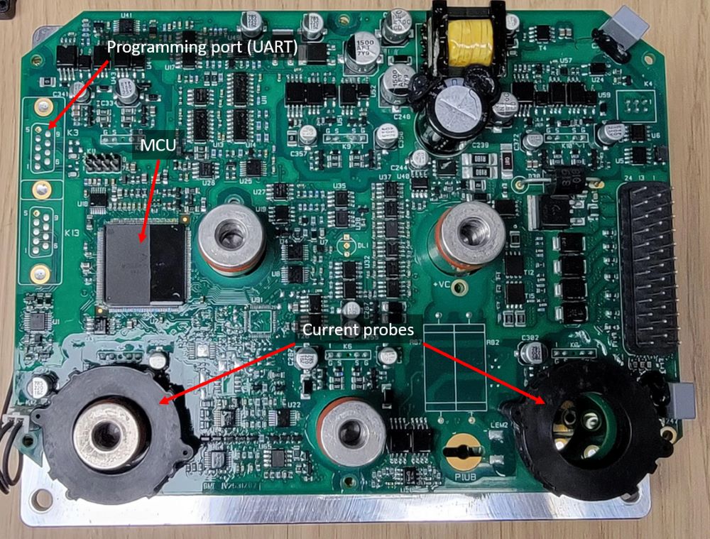
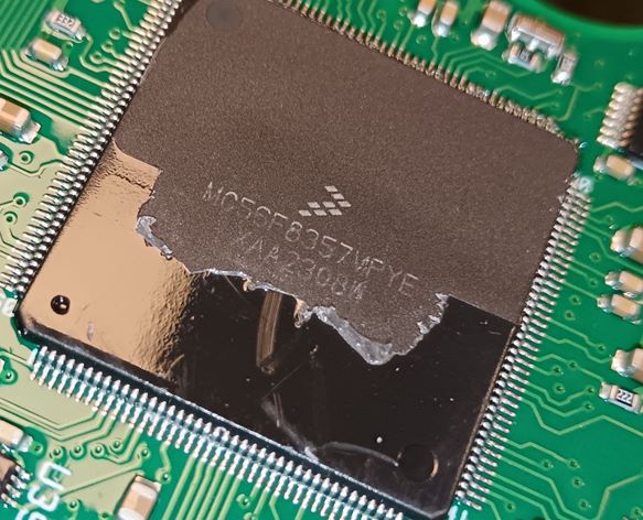 NXP MC56F8357VPYE
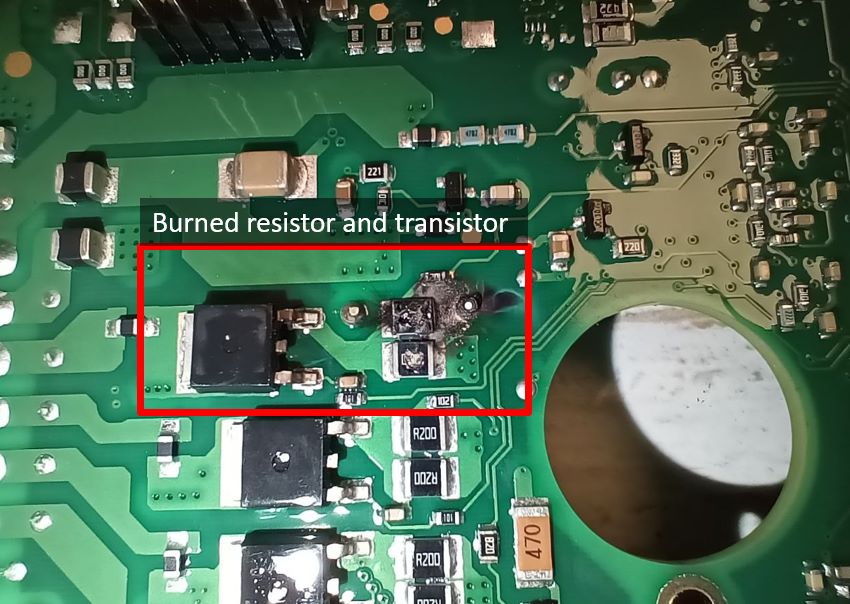
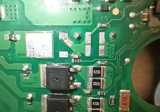
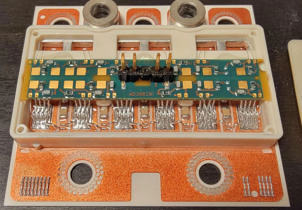
Since we have carried out an electrical installation for this inverter, all the wiring is the same as that of a Sevcon Gen4 as we can see below. The only thing worth mentioning is that it is possible to bridge the digital inputs to both GND and +12v positive when this is not possible in Sevcon Gen4.
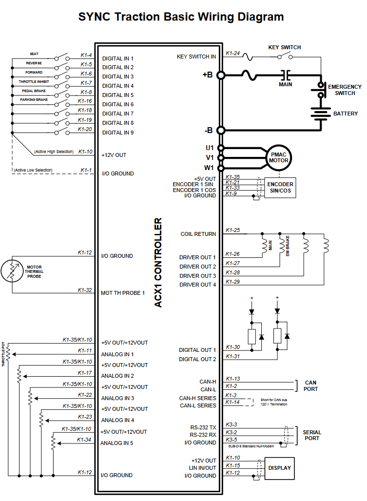 Dana TM4 wiring scheme
Software
To connect to the inverter, unlike many other brands that require specific and quite expensive hardware, we only need a generic USB-UART interface, so it’s a positive point for it.
The software is called SmartView PC Interface, developed with LabView 10 and is still the one initially programmed by SME, quite outdated although I don’t know if DANA has developed a new version. At least we didn’t get access to it.
It is quite well organized and its learning is very simple. The only drawback we saw is that during monitoring sometimes the connection with the inverter was lost and the interface was reset, returning to the initial screen of the program, something quite uncomfortable when you are working on it.
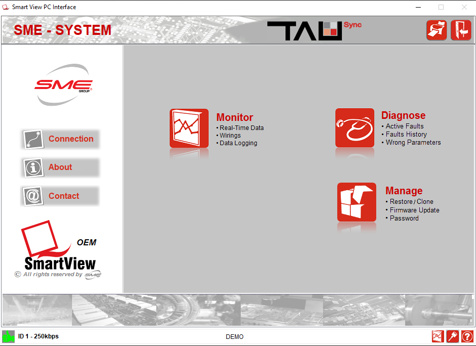
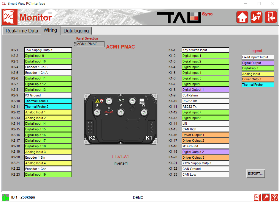 |
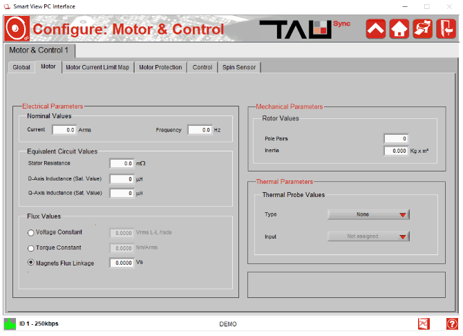 |
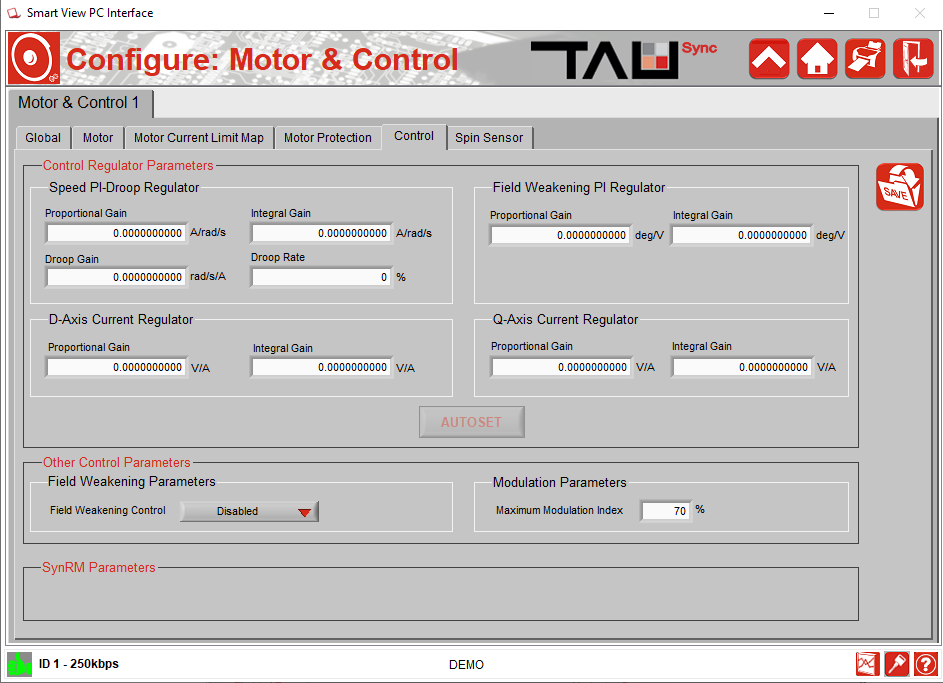 |
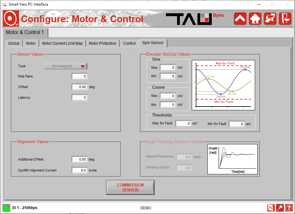 |
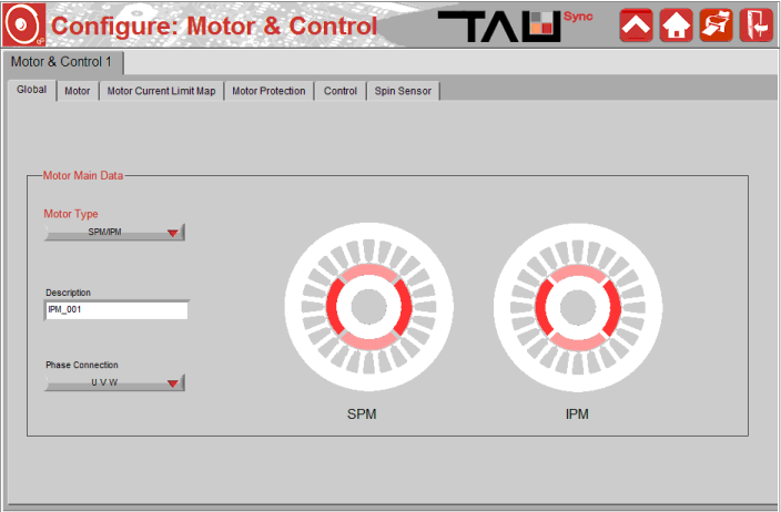
As you can see, another feature is that it allows changing phases from software in case they are not properly wired physically.
Sevcon Gen4 Size656
Tested: YES
Hardware
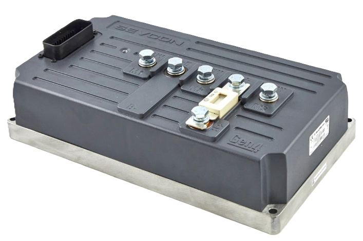 Sevcon Gen4 Size6
| Specification | Value |
| Input voltage | 50.4 to 96V |
| Maximum input voltage | 120V |
| Minimum input voltage | 39.1V |
| Peak phase current | 660A (2 min) |
| Continuous phase current | 210A |
| Switching frequency | 8 kHz |
| Sin/cos encoder support | Yes |
| IPM motor support | Yes |
Finally, we will analyze the Sevcon Gen4, now belonging to the Borgwarner company. We will focus on the Size6, the largest of its series, supporting 660A peak, an inverter that has surely given us many headaches.
We find an inverter that is already a few years old but is still quite competitive. It allows outputting 660A peak, which is more than enough for our application, although it’s true that it could lack some amps for the acceleration test. Recently, in the latest firmwares, they have raised the maximum working voltage from 116V to 120V, being close to the maximum 126V that the organization allows us.
At the hardware level, it should be noted that it supports sin/cos encoders, which meets the requirements of our application. It also has support for IPM motors through lookup tables and has a huge number of parameters for adjustment.
Obviously, not everything could be positive. The two major problems with this inverter are the lack of documentation for its parameterization and the impossibility of generating lookup tables for IPM motors. Regarding the first problem, the inverter has a large number of parameters which are not described in any type of document and the only way to understand what they do or what they affect is by trying and testing. Regarding the lookup tables, as we will analyze later, these are generated only by Sevcon, so either there are tables for the motor we are looking for or it’s “impossible” to generate them.
Software
IXXAT USB to CAN
The software used is DVT Customer, written in TCL/Tk.
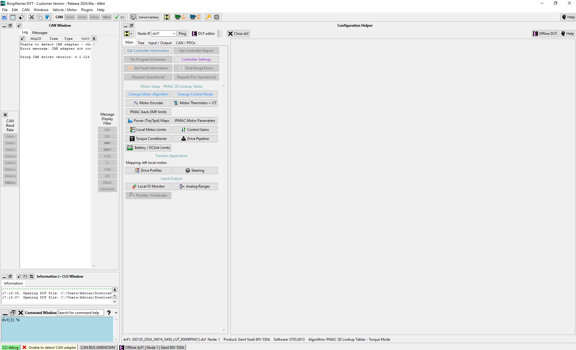 Main DVT screen
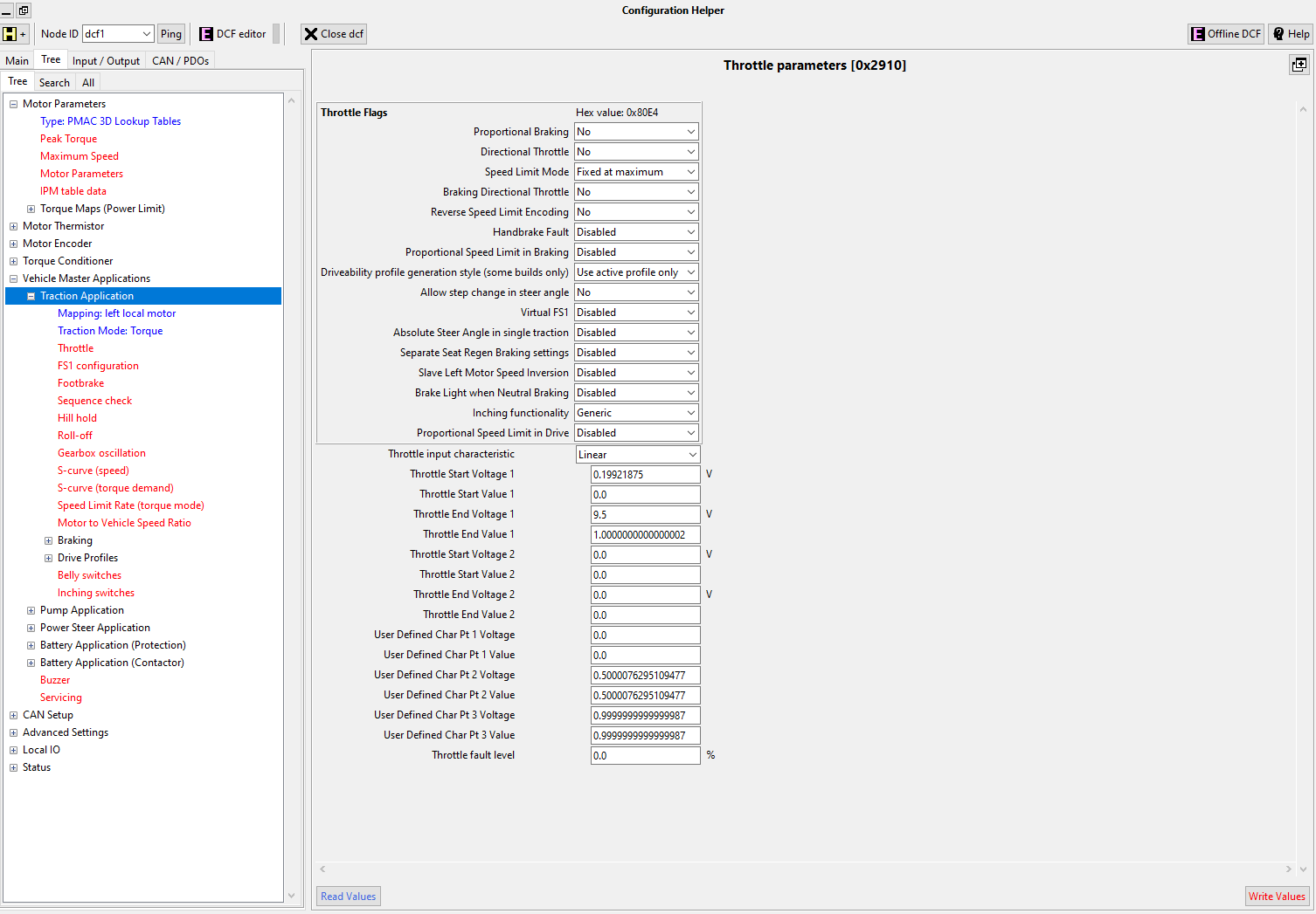 Throttle parameter configuration
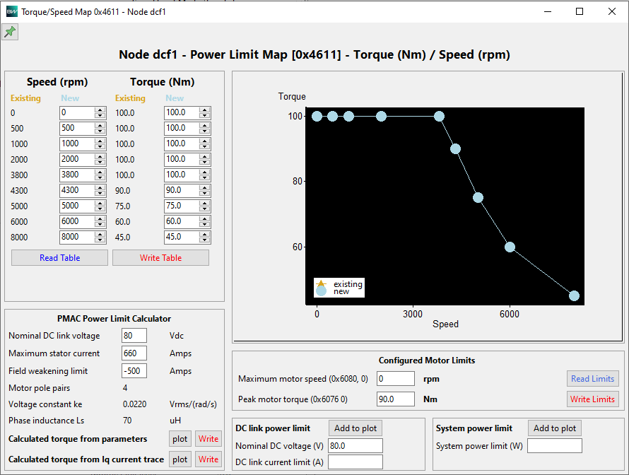 Torque limit map
The biggest problem I have found after working with it for hundreds of hours is that it does not have a real-time monitoring module for the inverter to be able to understand what is happening at that moment. We will also analyze this later.
How to Program Sevcon Gen4 💻
Introduction
After hundreds of hours of searching and reading in multiple forums, articles, documents and more, I have not found any manual or tutorial that expresses in detail how to program this inverter. I am not going to document again where each option is within the DVT program since there is documentation for that. I will try to reflect what I have learned on my own after hundreds of hours on the dyno trying to deduce what each parameter does and what it affects.
NOTE: I am not an expert in this field, there may be things reflected here that are incorrect or incomplete but it’s better to contribute something than nothing. If anyone reads this document and finds something wrong, incomplete or missing, please contact me to fix it.
Before starting with this, I consider it mandatory to read the document Gen4 LV size 2/4/6 Product Manual. This can be found in the DVT help in the latest versions or on internet: https://borgwarnerlugo.sharefile.com/share/view/s626b333e5dfd41e8997c28f2db195d65
On the other hand, it should be noted that in the DVT help we have a small guide for parameterizing the inverter that can help us as a starting point.
I will divide this section into 2 main parts, the theory about the control of these motors and the more “practical” part reflecting it in the DVT software.
Theory
The first thing we need to think about is what type of motor we are dealing with. In both cases mentioned above (ENGIRO and ME1616) we are dealing with a synchronous alternating current (AC) motor with internal permanent magnets. This is essential because it determines the algorithm that we must use in the inverter.
Within the Sevcon Gen4 Size6 models, there are at least two hardware models, one with support for sin/cos encoders (focused on PMAC motors) and another for induction motors with other types of encoders. This will also be reflected in the firmware that the Sevcon has internally, so it’s important when purchasing one.
The motor is powered by 3 phases. These three phases receive alternating current (a sine wave), with a phase shift of 120 degrees between them.
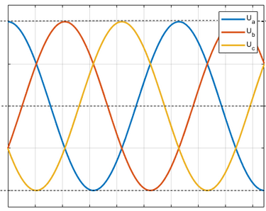 Example of 3 phases
Controlling the 3 phases is complex, so there are strategies for simplifying and managing them, as we will see below.
FOC Algorithm & Vector Control
Depending on the frequency, amplitude, etc. of the wave, the motor will rotate at a certain speed or have a certain torque (it’s a bit more complex than that). Remember that this motors have permanent magnets inside, so the rotor will be synchronized with the frequency generated on the stator. This 3 phases can be represented as vectors to control the motor. The control of these 3 vectors is somewhat complex, so we have the FOC (Field Oriented Control) algorithm.
Trying to explain in a simple way, this algorithm simplifies the handling of the 3 vectors (the phases) into 2 static vectors to the rotor. For this purpose, it uses the Clark and Park transforms. This two vectors generated are Iq and Id. The Iq vector manages the torque and the Id vector manages the magnetic flux as we can see below.
The commercial inverters have the vector control and FOC implemented and each implementation is a little different. I am going to try to explain it in a simple way, although probably incorrect in some points.
As we can see, the process starts with the 3 phases. By applying the Clark transform, we can simplify the 3 signals, one for the torque and another for the magnetic flux.
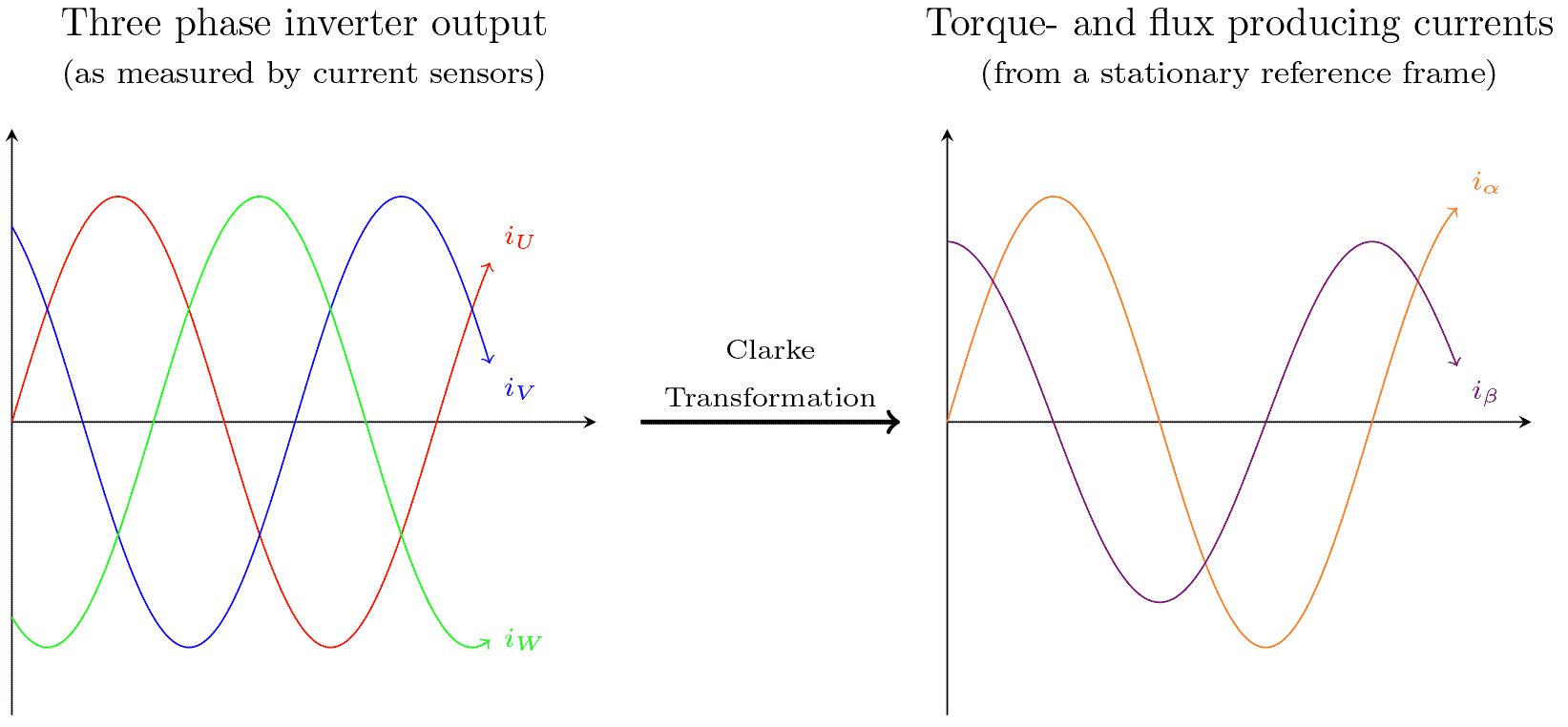 First step: Clark transform57
The Park transform is then applied to change the vectors from a stationary reference (the stator) to a rotating reference (the rotor).
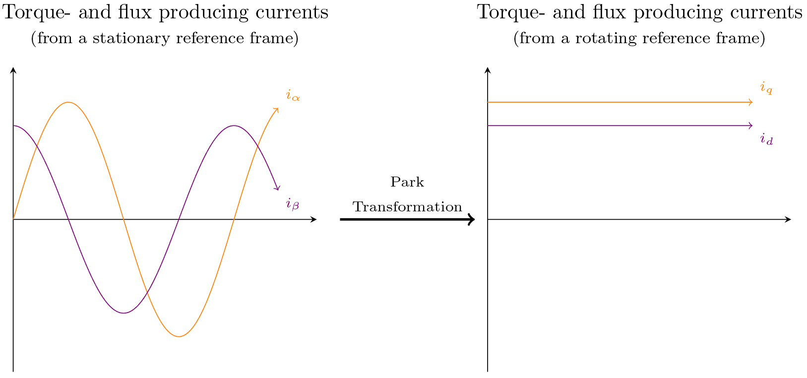 Second step: Park transform57
These two vectors are much easier to control, one representing torque and the other representing magnetic flux. Let’s look at the full example. The inverter measures the current of the motor phases, performs the transformations and obtains the Id and Iq axes. Regarding these axes, it makes the changes through the control loop and again transforms these two vectors into the 3 phases of the motor.
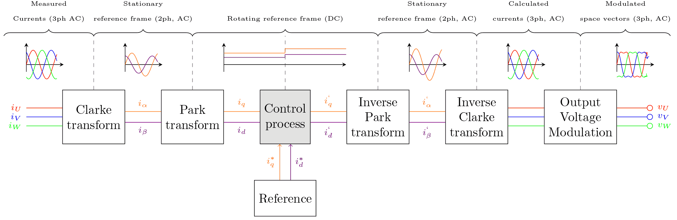 Complete process57
Below we can see how the process is simplified:
 Complete process57
You can read more about it here: www.switchcraft.org/learning/2016/12/16/vector-control-for-dummies
Note that these algorithms were developed many years ago, but the computation capacity of the systems was not sufficient to do it in real time until a few years ago. The positive part is that we don’t need to understand in detail how this process occurs as it’s already implemented by manufacturers of the inverters. Thanks to it we can focus only on the handling of the two vectors:
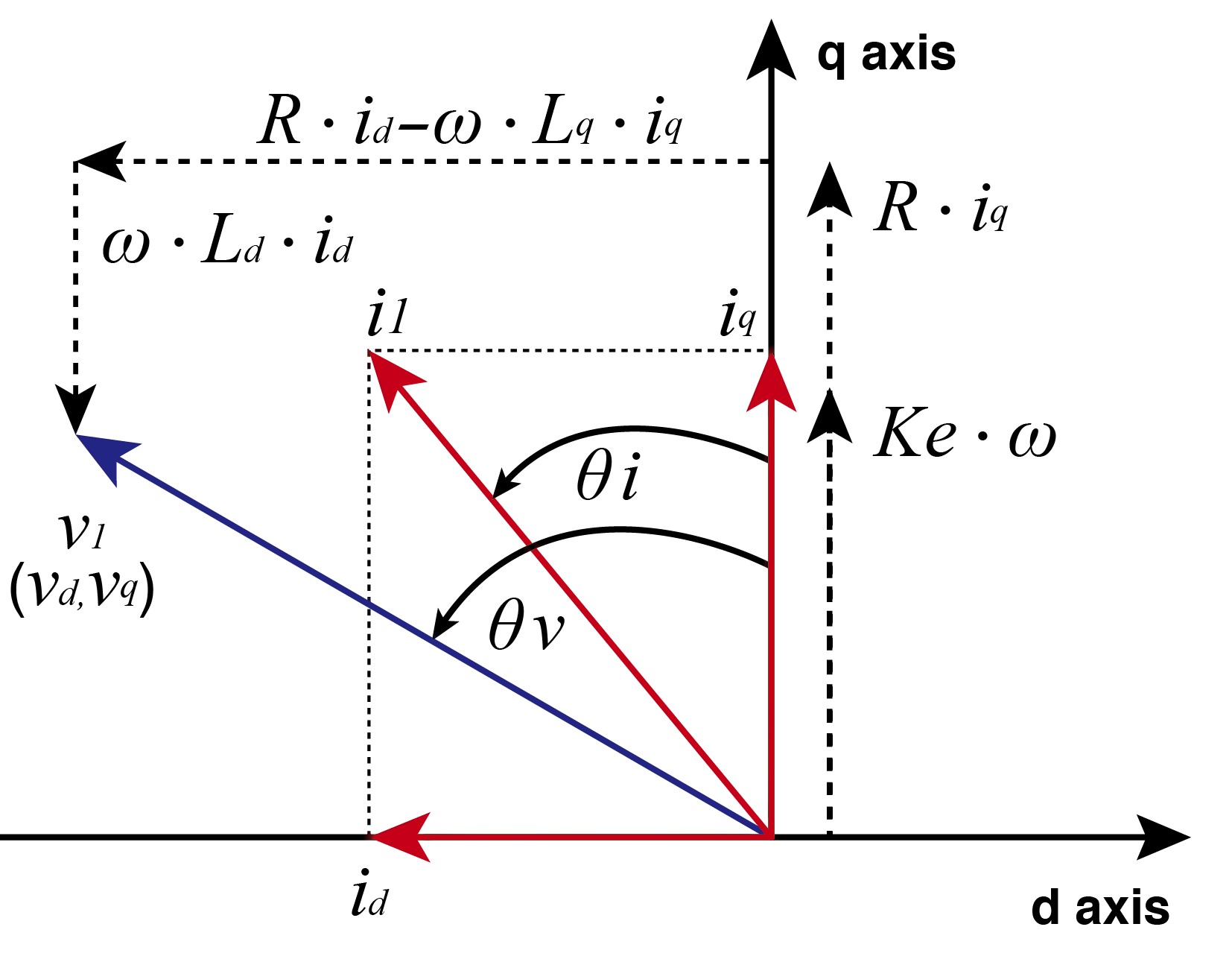 FOC Vectors58
The Iq vector on the vertical axis and Id vector on the horizontal axis. Note that Id is negative. We will explain it later. It’s also important to understand the resulting current:
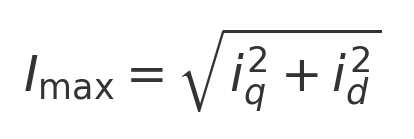
Which means that if we want to apply current on the D-axis, we must decrease it on the Q-axis and vice versa, always keeping in mind to find the maximum resulting vector.
Until now we have talked about the control vector. Below is an example of the complete FOC algorithm:
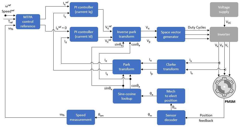 FOC Control59
To understand it, we need more basic concepts.
Field Weakening
Remember that we are talking about motors with permanent magnets in the rotor. In order for it to work, we induce a magnetic field with the coils in the stator, which causes the rotor to spin. By having magnets, the rotor itself induces a magnetic field back on the coils, which generates a voltage back on the phases of the motor. This is what is known as the Back-EMF or counter electromotive force.
This Back-EMF is directly proportional to the revolutions of the motor with a constant current. This means that there is a moment when the motor produces a Back-EMF so large that it’s equal to the voltage with which the inverter is driving the motor. This prevents the motor from being able to rev higher. This point is known as the base speed.
Once the base speed is reached, theoretically the motor cannot run at higher revolutions. We could say that it slows itself down. This is when the Field weakening or Flux weakening technique comes into play.
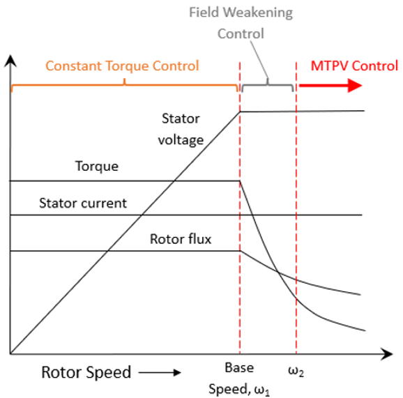 Field weakening graph60
This technique of field weakening consists of reducing the magnetic flux induced by the magnets on the motor coils, trying to make the Back-EMF smaller and therefore, being able to raise the motor to higher revolutions than theoretically possible. This is done by shifting the magnetic field.
This is achieved by playing with the Iq and Id vectors that we have seen previously. When the motor starts (SPM), we must apply all the current to the Iq vector so that generates torque on it. When the motor has reached the base speed and cannot increase its revolutions any further, we must start applying field weakening. This means that we begin to introduce current into the D-axis, reducing the torque applied to the Q-axis but allowing the motor to increase its revolutions. Remember that Power = Torque x revolutions.
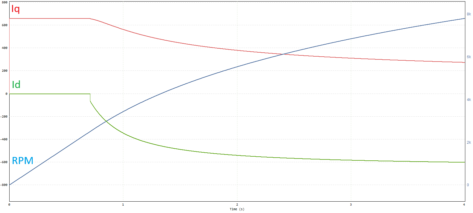 Field weakening example
As we can see, the motor starts to rotate by applying all the current to the Q-axis. When the base speed is reached, we start to apply current to the D-axis (and therefore decreasing it on the Q-axis). In this way we manage to increase the motor revolutions above the base speed. This strategy is known as field weakening.
It should be noted that the application of field weakening has two disadvantages, the first is that it increases the temperature of the rotor, which we have to be careful with since if the temperature rises too much we can demagnetize the magnets. On the other hand, if we introduce too much current into the D-axis, we can demagnetize the rotor too, breaking the motor.
But what exactly does field weakening mean in the motor? How does it work? After analyzing the sinusoids in PSIM software, simulating the motor and control system, I could not see any significant change in the amplitude or frequency of the waves/signals that drive the motor. I decided to introduce a resolver to check the phase shift:
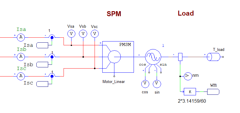 Modified SPM model on PSIM
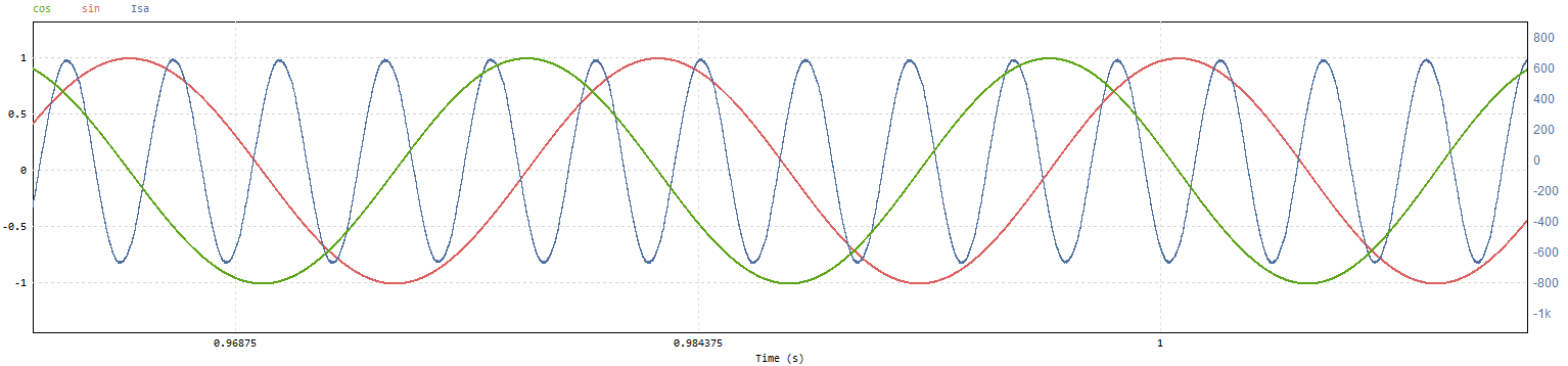 Sine, cosine and phase waves
We can see the cosine signal leading sine signal. We are going to remove the sine signal for a cleaner view. After measuring the data I got this results:
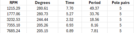 Field weakening starts before 3232 RPM. Note the degree change on after that speed
Field weakening causes the wave to shift in phase with respect to the motor position, advancing it in degrees.
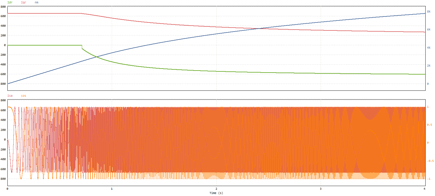 Field weakening
When Id is 0, the degrees between cosine signal and phase A are the same even if the RPM change. When field weakening is applied, the wave starts shifting as you can see on the table. Could we say that it is like an ignition advance in a combustion engine?
Inductance & Reluctance
TO-DO
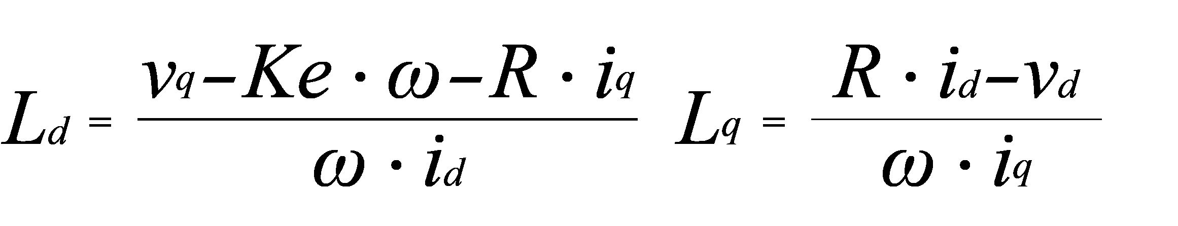 Ld and Lq inductances58
MTPA (Most Torque Per Ampere)
As we have seen previously, the inductances on the D-axis and Q-axis are different in an IPM motor. This means that to obtain the highest torque in an IPM motor, we must not only apply current on the Q-axis but also on the D-axis from the beginning.
This is what is known as MTPA. It consists of injecting current into the D-axis from the beginning, increasing the torque of the IPM motor compared to the traditional technique. Below we can see an example:
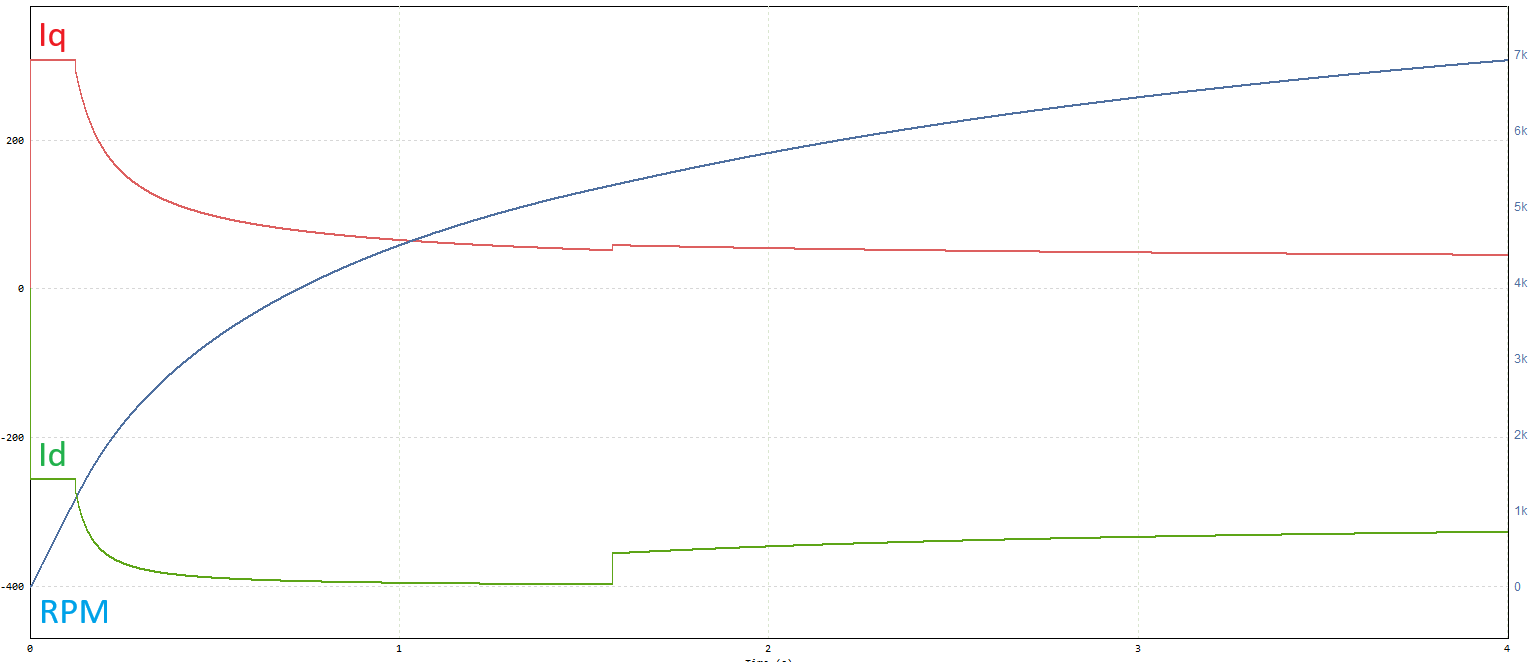 MTPA Example
Current is applied to the D-axis from the beginning. Once the base speed has been reached, it will continue working with the field weakening strategy, as in an SPM motor.
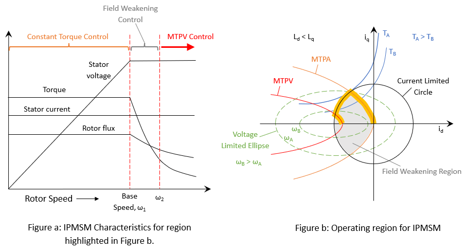 MTPA Algorithm60
In the figure b, the yellow path is the one that we should follow to obtain the maximum performance of a motor. We would start by applying current on the Q-axis and on the D-axis, and progressively moving it to the D-axis, following the MTPA curve. Once we have reached the limit of the resulting current, we will begin to apply the field weakening strategy, moving a greater amount of current to the D-axis until reaching the MTPV curve.
There are two options to implement MTPA:
- 3D Lookup Tables: This consists of defining tables in which we indicate the Iq and Id values in relation to the revolutions, torque requested and voltage. In this way we can establish values that the inverter will take to follow the MTPA curve. Some of the inverters that use this system are the Sevcon Gen4 and the DMC.
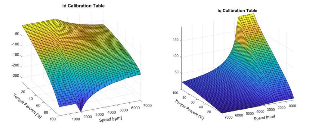 Example of 3D lookup tables61
- Polynomic Function: This consists of establishing a polynomial that describes the MTPA curve, in such a way that the inverter can follow it based on dynamic values. EmDrive applies this strategy:
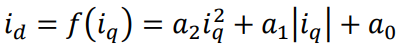 EmDrive MTPA polynomic function41
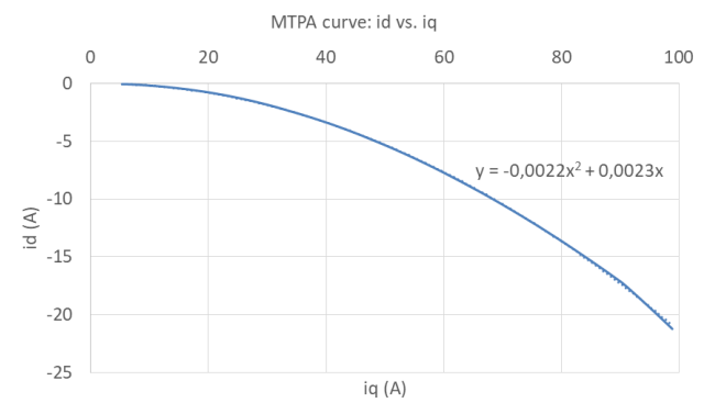 Graphical representation41
PIDs (Proportional-Integral-Derivative Controller)
A PID controller (Proportional-integral-derivative controller) is a feedback control system used to adjust the output of a system to maintain a desired setpoint. It continuously calculates and applies corrections based on the feedback signal.
The question is, why do we need a PID? Mainly because we are handling a signal that is not the same as the one we are receiving feedback with. Let’s take an example, a water tank that has a resistor to heat up. The tank will have a temperature sensor. That temperature sensor gives us feedback in degrees Celsius for example, but we are handling a resistor. The system has inertia and delays so we will need a PID to adjust it. Similarly, the cruise control of a vehicle, we have a speed feedback, which is also our setpoint, but we are handling the torque or accelerator of the vehicle.
In this case, this inverter have multiple PIDs. Specifically, Sevcon has PIs, so it does not have the derivative part of control. Some of this PIs are:
- Speed Control: If speed control is enabled or a speed limit is introduced for the motor, a PI will start to operate in charge of controlling that speed. In this case we have a setpoint/feedback which is the motor speed and the signal that is managed is the torque applied to the motor.
- Torque Control: In both torque and speed mode, the inverter uses a PI to control the current. This is because the inverter modulates the voltage entering the motor and the setpoint and feedback are currents. As we will see later, with the FOC algorithm we manage the currents on the Iq and Id axes. We have the current feedback in two of the phases that feed back the system.
In Sevcon, the PI is parameterized with two values, Kp and Ki. Below we can see an example of a well-configured PID and another PID with overshoot.
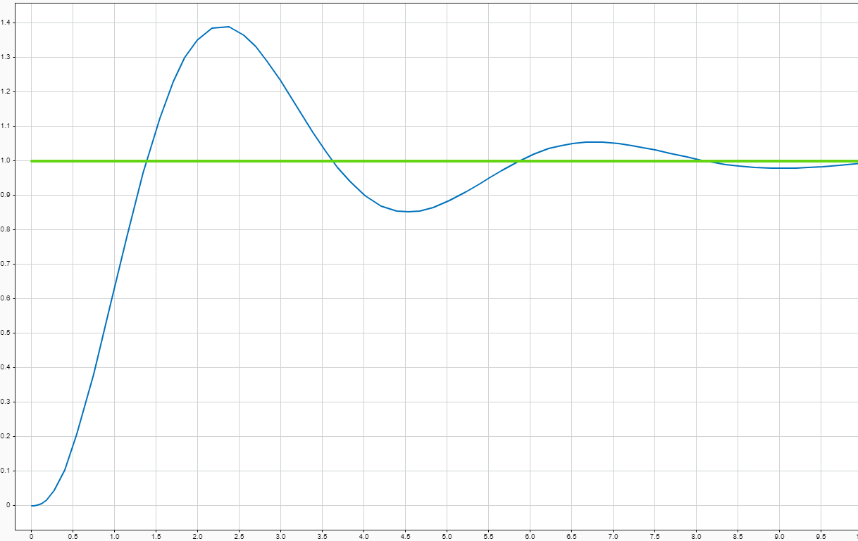 Incorrect PID tune |
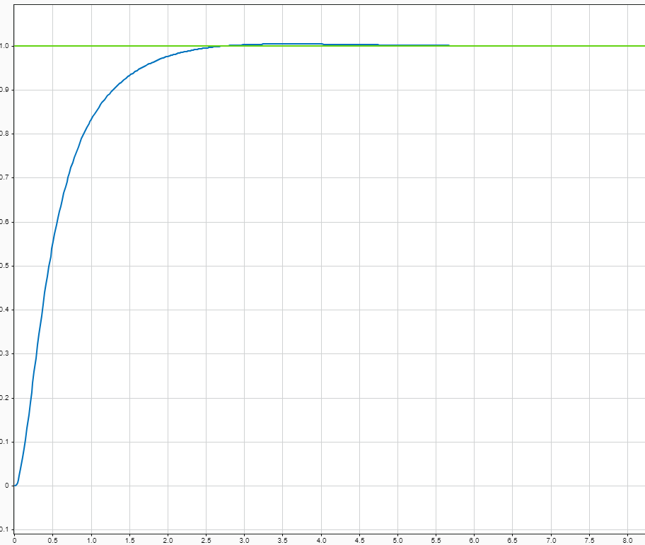 Well tuned PID |
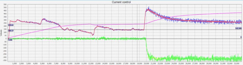 Example of current control on Iq and Id axis.
Switching Frequency
The switching frequency is the rate at which the transistors or IGBTs turns on and off to control the flow of the electrical power from the DC to the AC for the motor. It’s measured in Hz, representing the number of times the switches toggle per second.
The first thing we need to understand is that we have a DC current source that we need to transform into AC. We must bear in mind that the DC current we have does not have negative voltage, and that the AC current we are going to generate needs to have a negative component.
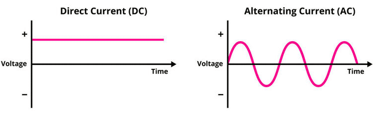 DC vs AC62
For this, the six-step inverter is used. With this we manage to generate a sine wave. 3 of the transistors are used to generate the 3 positive waves of the phases and the other 3 transistors are used to generate the 3 negative waves of the phases.
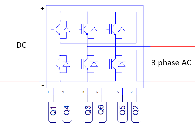 Six step inverter example63
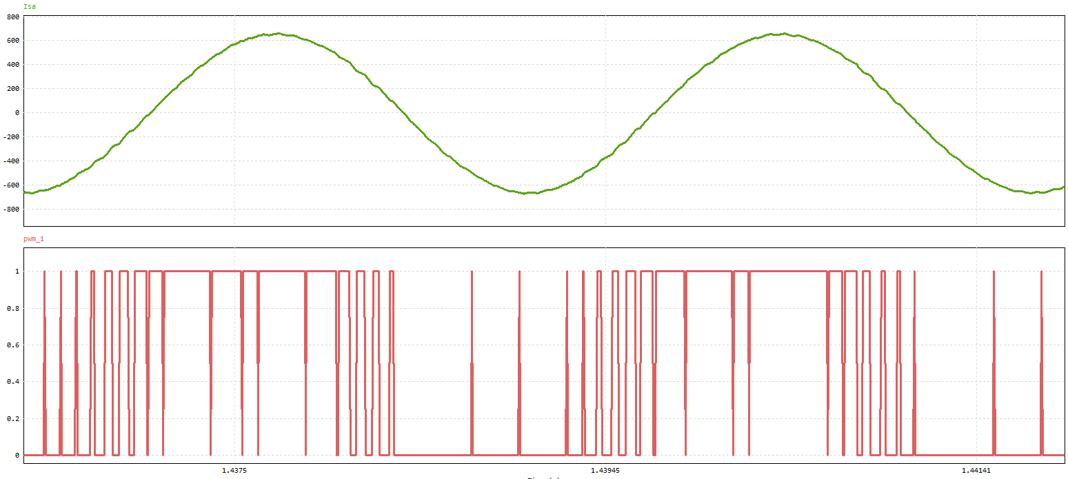 PWM signal and sinusoidal signal
The PWM modulation has a constant voltage and what changes is the time that the signal is HIGH or LOW (what is known as the duty cycle). The longer the duty cycle, the greater the current flow of the transistor. By performing this fast switching, we obtain a sinusoidal output signal (we could say that the average of the current is generated wave).
In this way, the inverter is able to convert the DC current into AC to drive the motor. It should be noted that the higher the switching frequency, the higher the quality of the sine wave generated. However, a higher switching frequency also heats up the transistors.
However, a low switching frequency, although it heats the transistors less, will generate a lower quality signal, which will produce unexpected behaviors and a non-constant torque in the motor. Below we can see a signal with a low switching frequency.
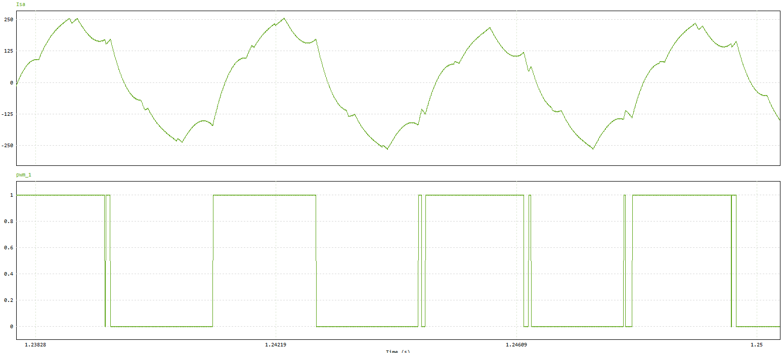 Low PWM switching frequency
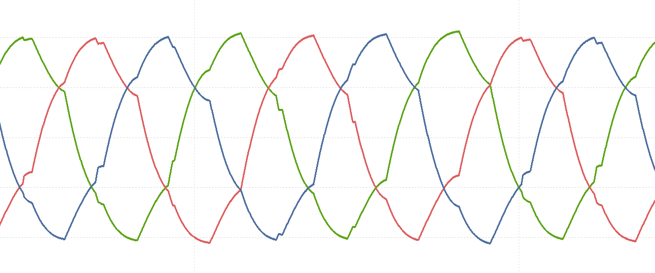 Low switching frequency
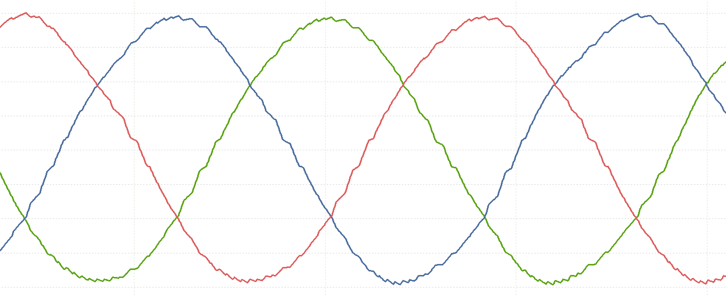 Medium switching frequency
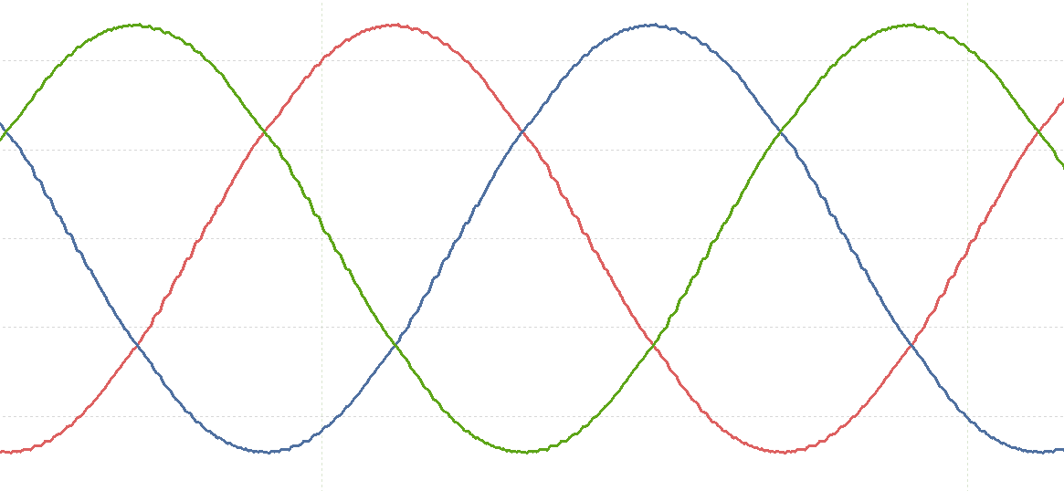 High switching frequency
Below we can see an example of the generation of the sinusoid with the six step inverter:
 Example of 6-step inverter working
Drive Modes
Once we have a clear idea of what MTPA, field weakening and the FOC algorithm are, we can move on to the control part. This part is responsible for ensuring, in a general summary, that the motor receives the current that we demand.
This type of inverters for traction motors usually have two driving modes:
-
Torque Mode: In this mode, the throttle directly controls the torque delivered by the motor, like the accelerator of a thermal engine.
-
Speed Mode: In this mode, the throttle indicates the speed at which the vehicle must go. The inverter is in charge of managing the torque necessary to reach that speed. This could be compared to the cruise control in cars, in which we set a constant speed and the control unit is in charge of, for example, accelerating the vehicle if we reach a hill to keep the speed.
Understanding everything together
With all the above mentioned, let’s try to understand the complete FOC algorithm with the following scheme:
FOC control59
We can see how the algorithm takes the throttle position as an input value (Tref), which directly drives the torque/current we want to apply. With this information, it applies the MTPA or field weakening depending on the speed of the motor and the current demanded. This will generate a specific Iq and Id which we want to apply to the motor. These values go through a PI loop. Normally there are two PIs, one for the Q-axis and one for the D-axis. We can use the same Kp and Ki for both, or each one can have its own independent ones. We must bear in mind that the inverter modulates the input voltage to the motor (Vq, Vd), which is why we have the PI loop. This, with the feedback of the current measured in two of the motor phases (after performing the Park and Clarke transformations), adjusts with respect to the reference currents we want in each of the axes.
After that, the system is fed back, recalculating the voltage needed by the PI to meet the requirements of the reference signal and then the inverse of the Park and Clark transforms are performed to generate the 3 vectors that result in the 3 phases of the motor. The system is fed back with the encoder, knowing the position of the motor rotor at all times and the space vector generator is responsible for generating the PWM signals that will manage the inverter transistors as we have seen previously.
As we can see in this other graph, the basis of any system like these is torque control. From there, layers such as speed control or position control are implemented, each with its corresponding PI controllers.
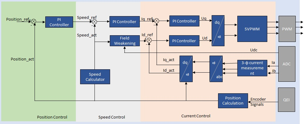 Multiple controls
IPM vs SPM Control
As discussed earlier, there are two types of permanent magnet motors: SPM (Surface Permanent Magnet) and IPM (Interior Permanent Magnet). Besides differences in construction and characteristics, the control strategy for each motor type also differs. The control method for an SPM motor can be used on an IPM motor, but it won’t deliver optimal performance. The key distinction is that an IPM motor requires the MTPA (Maximum Torque per Ampere) strategy to achieve the highest possible torque.
 IPM control with MTPA
 SPM control without MTPA
In the first example, current is applied to both the D-axis and Q-axis following the MTPA curve. Once base speed is reached, field weakening is applied. In contrast, in the SPM example without MTPA, all current is initially applied to the Q-axis, and field weakening is applied after reaching base speed, similar to the IPM motor.
With this theory clear, we can now focus on programming the Sevcon inverter.
Programming Sevcon Gen4
Let’s get down to the most complex part. The theory we have seen above is nice, but the main problem I encountered when programming the inverter was the lack of documentation and description of certain parameters. It’s clear that the manufacturer is interested in companies sending them the motor to be characterized and not having it done by people outside of them.
I’m going to divide this section into the following blocks:
- Phase order: Mounting the phase cables in a proper order.
- Input and output configuration: Configuration related to inputs such as the throttle or buttons and outputs such as the contactor or throttle voltage.
- Motor parameterization: All the configuration related to the motor, encoder, temperature sensor, etc.
- Control parameterization: Configuration related to the speed, torque, PIs and more.
- Behavior parameterization: Configuration related to the throttle response, battery between others.
- Safety configuration: Setting maximum values such as motor revolutions or currents.
- Advanced settings: Other advanced inverter settings
Phase Order
The first thing we must do before starting the motor is to connect the phases in the correct order. The Setting up PMAC software document explains how to do this. The inverter has 3 connections for the 3 phases of the motor, M1, M2 and M3.
Before performing this step, we must make sure that we have the encoder configured correctly. This can be seen in the “Encoder setup” section below.
Now, with the voltage and inputs set correctly, we can connect the encoder with only the 5V and 0V terminals and turn on the inverter. This will cause the encoder to be powered and produce an output signal.
If we rotate the motor forwards, we should see the cosine signal leading the sine signal as we can see here:
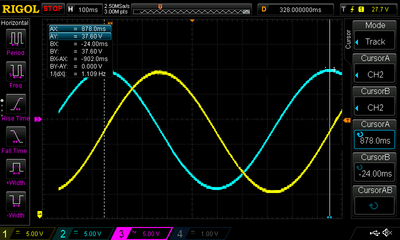 Cosine (blue) signal leading sine (yellow) signal
This means that channel 2 (cosine) must be connected to pin 35 and channel 1 (sine) must be connected to pin 31. If you want to make the motor rotate backwards, you can invert this signals. The decision must be taken before phase order calculation.
The motor phases are 120 degrees shifted between them. With that, we can start measuring the phase shift between the encoder and each of the phases. To do this, using the oscilloscope, we will change one of the probes between each of the phases, attaching the GND connection to the next phase as can be seen below:
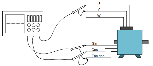 Phase connection64
The motor can be rotated by hand or use a drill. We should get something like this:
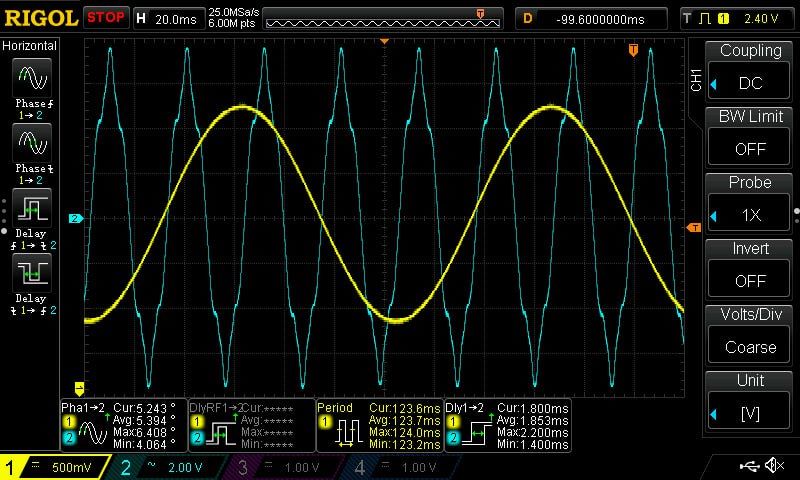 Cos and first phase
Now we need to measure the period of the encoder signal:
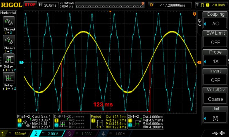 Signal period
And the time between the start of the cos and the start phase wave:
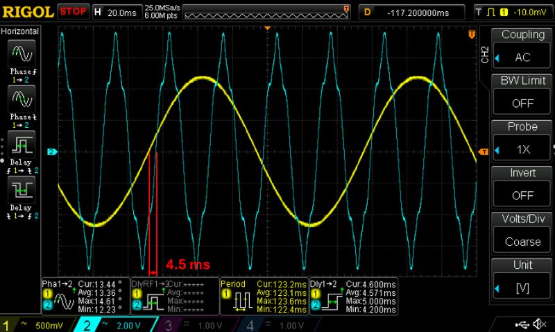 Time between two signals
To calculate the angle, we use this formula:
We must perform this calculation for each of the phases. With the three angles calculated. Then select the angle closest to 0 degrees.
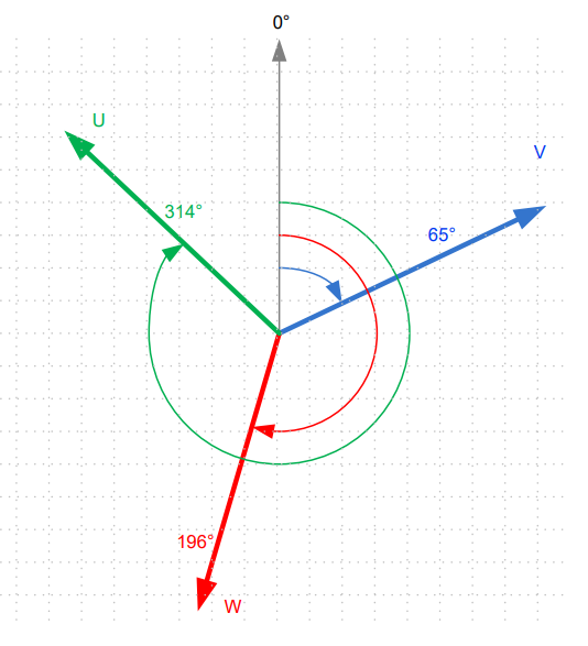 Phase shift64
The measurement should give us a distance between each of the phases close to 120 degrees. If this is not the case, the measurement is incorrect. With this data, we can place the phases in the correct order, starting with the one closest to 0 degrees and continuing in clockwise order.
Electrical vs Mechanical Angle
In an electric motor we have two angles, the mechanical angle and the electrical angle.
- Mechanical angle: Corresponds to the mechanical rotation of the motor and the encoder signal.
- Electrical angle: Depends on the number of pole pairs of the motor.
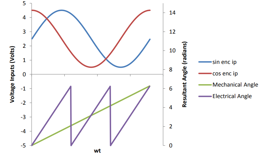 Electrical vs mechanical angle64
As you can see in the image below, the encoders of electric motors are usually artificial and can be moved. Let’s imagine that in a 4-pair pole motor, we have the phases U, V, W in order with an initial angle of 20 degrees between the 0 of the encoder and the U phase.
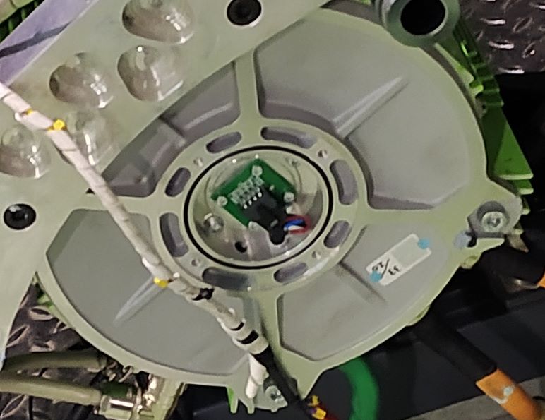 Engiro encoder
If we rotate the encoder physically by 90 perfect degrees, without touching the rotor, we will be back at the same phase angle (20 degrees) with respect to the U phase.
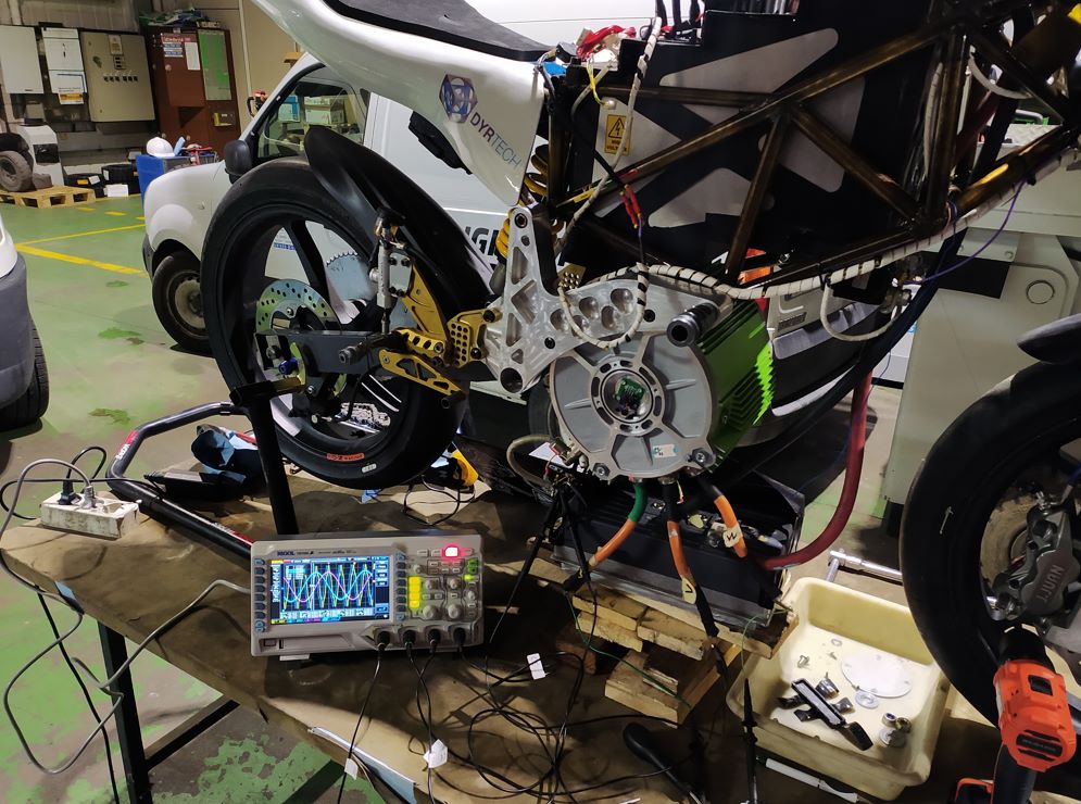 Analyzing signals
DVT Software
There is also a DVT software manual so it is recommended to read it to understand where each of the options are located in the program. Here you can find it: https://borgwarnerlugo.sharefile.com/d-s03b47c020329497a9ec94c9c01e776ed
To locate the parameters, a hexadecimal index is used, as a kind of key-value dictionary. It has a format of 0xAAAA, bit. Once configured CAN connection properly with the correct speed, we can connect and see this menu:
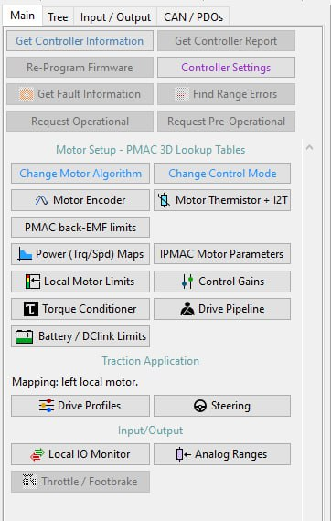 DVT main menu
We have this window in which we should mainly focus on the tabs:
- Main: Tab for the basic configuration of the inverter.
- Tree: Tab with all the parameters of the inverter.
- Input/output: Configuration of the inputs/outputs of the inverter.
- CAN/PDOs: Configuration of the CAN PDOs.
Input and Output Configuration
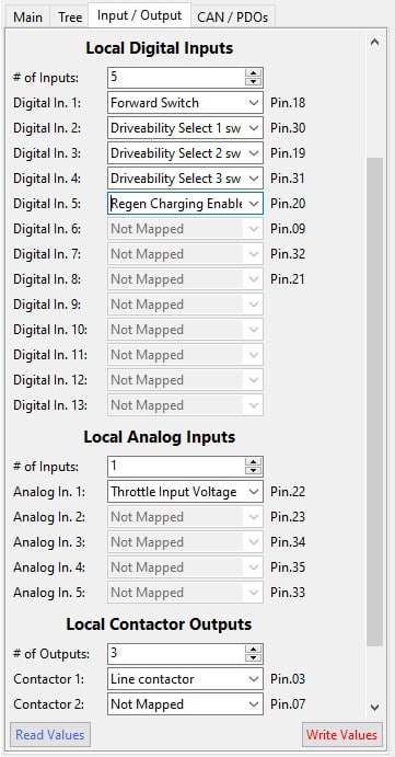 DVT input configuration
We need to start by configuring the inputs/outputs. This will vary depending on the connections we have made in the wiring installation. Basically we have 3 sections:
- Local digital inputs: We will configure the Forward switch to indicate when we want the traction to be activated, 3 driveability to configure different power maps/configurations based on the 3 buttons we have on the handlebars (optional). Finally, we will configure an input to enable regeneration (optional). In this example, it corresponds to the throttle interlock (a switch that is closed in the rest position). At least Forward must be configured.
- Local analog inputs: Analog inputs. We will only use the throttle.
- Local contactor outputs: For our application we will only use one contactor.
Before starting the inverter, we must also configure the encoder and contactor supply voltages. This is important before starting the inverter, since we can break both elements in case of having a high voltage.
Contactor Voltage
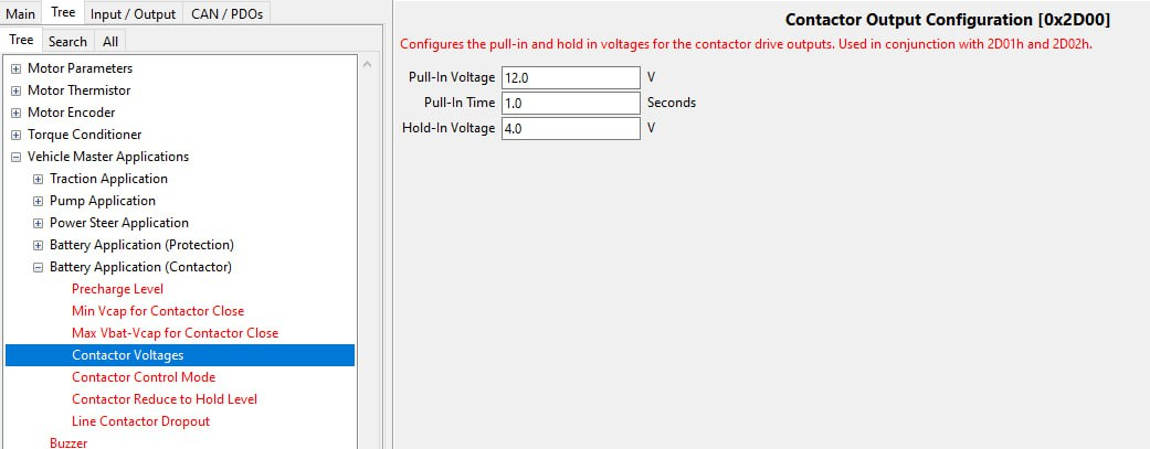 DVT contactor configuration
- Pull-In voltage (V) (0x2D00,1): This is the initial voltage with which we make the contactor close. We can set the nominal voltage or a little higher. If we test with different voltages, we can see that as we lower the voltage, the contactor makes less noise when it closes. The ideal voltage would be the nominal voltage, or a bit higher.
- Pull-In Time (s) (0x2D00,2): This is the time that the Pull-In voltage will be maintained. One second is more than enough.
- Hold-In Voltage (V) (0x2D00,3): This is the voltage at which the inverter will keep the contactor closed. We must test and check the temperature of the contactor coil. Ideally, the voltage should be slightly below the nominal voltage to prevent it from overheating, but if it’s too low, we have the risk of not having enough power to keep the contactor closed. It’s best to consult the manual of the installed contactor.
Encoder Setup
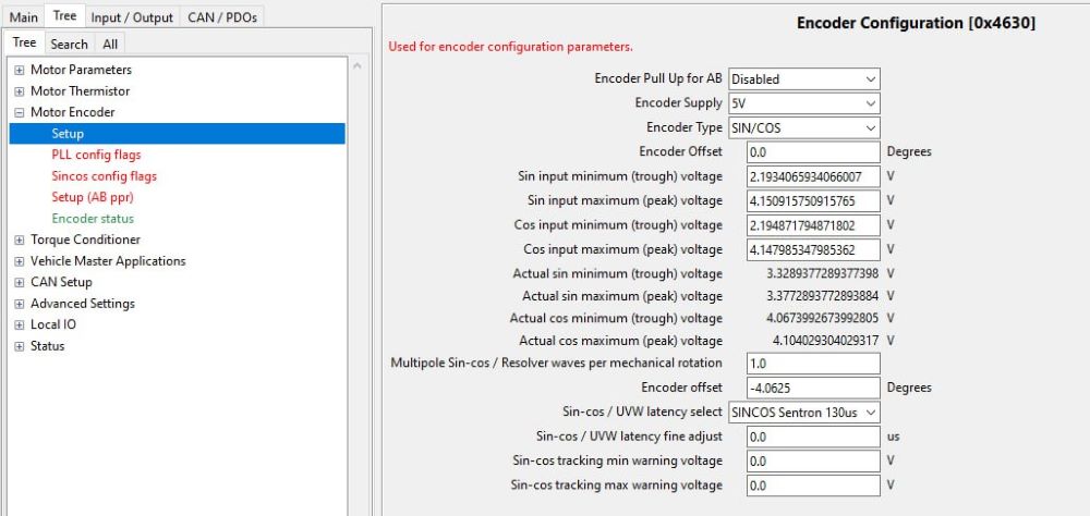 DVT encoder configuration
As with the contactor, we must select the voltage at which the encoder works. Sevcon has 2 voltages, 5V and 10V. We must select the one indicated by the manufacturer and the following options:
- Encoder Supply (0x4630, 3): 5V or 10V, based on manufacturer data.
- Encoder Pull Up for AB (0x4630,1): Must be Disabled.
- Encoder Type (0x4630,3): sin/cos.
- Encoder Offset (degrees) (0x4630,4): This will be set later.
- Sin-cos / UVW latency select (0x4630,18): Encoder latency based on manufacturer.
- Sin-cos / UVW latency fine adjust (us) (0x4630,19): This will be added to the previous parameter for fine adjust.
We will leave the last two with 0.0 by default.
After this, we must perform a commissioning of the encoder. This consists of the inverter reading several complete oscillations of the sine and cosine signal and establishing the maximum and minimum values. It’s a kind of calibration. To do this we simply have to rotate the motor by hand or with a drill and click on commission.
TO-DO: COMISSIONING
After this we will obtain the following updated values:
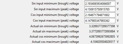 Encoder measured data
Throttle Setup
On the Main tab, click on Throttle/Footbrake setup. It will ask you to put the throttle on the maximum position and then back to rest position. This is because the inverter needs to know the voltage of the throttle at rest position and at maximum position.
We can also set these voltages manually in the following window:
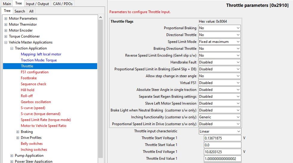 Throttle configuration
We can define manually the throttle voltages for the start position (0.0) and end position (1.0).
On the other hand, we can see in Throttle input characteristic (0x2910,2) how we can configure different curves for the throttle. These are Linear, Curved, Crawl or User Defined.
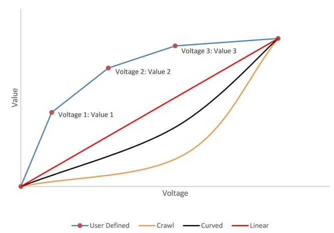 Throttle profiles65
If we want a user-defined curve, in the same window we have the textboxes to enter the values.
Motor & Static Data Parametrization
In this section we will try to configure all the elements that are given by the manufacturers or by the installation that we have, such as the motor data, battery between others.
This configuration will be different depending on the motor algorithm.
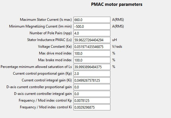 DVT SPM motor data
- Maximum Stator Current (Is max) (A) (0x4641,2): Maximum current supported by the motor stator. This data must be provided by the motor manufacturer.
- Minimum Magnetizing Current (Im min) (A) (0x4641,3): It’s the minimum current that we are going to apply on the D-axis (remember that it’s negative). We must be careful because applying too low a current can demagnetize the rotor.
- Number of Pole Pairs (npp) (0x4641,5).
- Stator Inductance PMAC (Ls) (uH) (0x4641,10): Stator inductance in μH. Used only for the geometric algorithm. It can be measured with a LCR.
- Voltage Constant (Ke) (V/rads) (0x4641,18): TO-DO
- Max drive mod index (%) (0x4641,30): TO-DO
- Max brake mod index (%) (0x4641,31): TO-DO
- Percentage minimum allowed saturation of Ls (%) (0x4641,43): TO-DO
The rest of the parameters belong to the control part that we will see later.
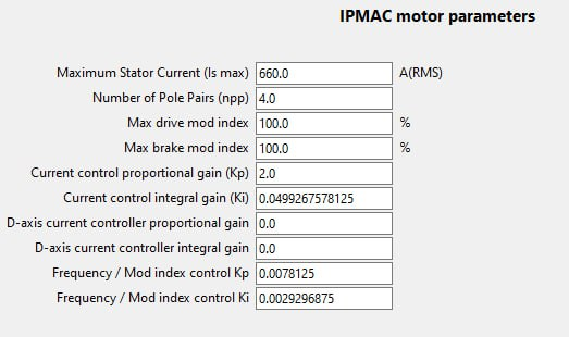 DVT IPM motor data
As we can see, the configuration of the IPM motor is simpler since some of the parameters are not necessary for the calculation of values that are already in the tables.
Speaking about the max modulation index, here you can see some results from the dyno with all the parameters equal except that one.
Max Mod Index 50
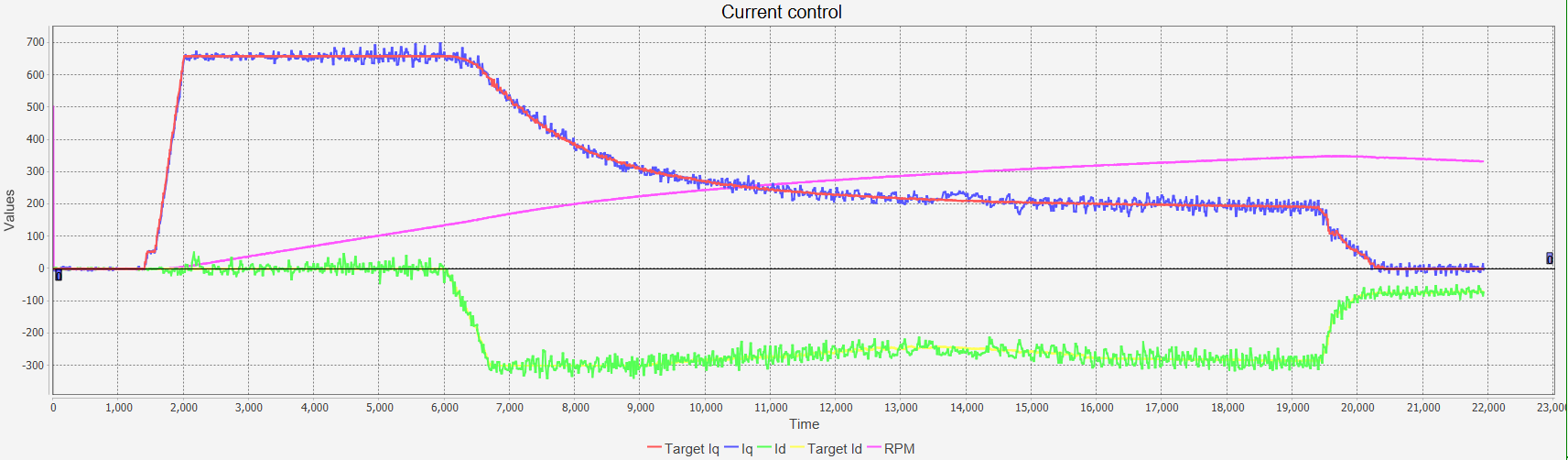
Max Mod Index 95
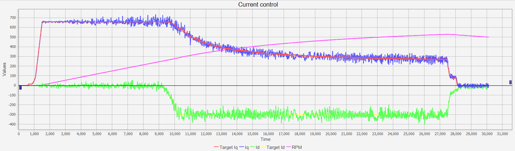
Max Mod Index 120
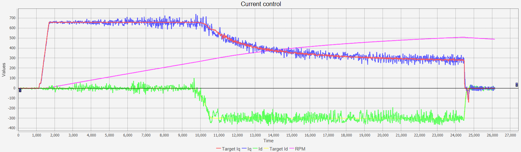
Control Parametrization
In this section we will configure the parameters related to the control, mainly to the PIs.
We can mainly distinguish 3 controls:
Current Control
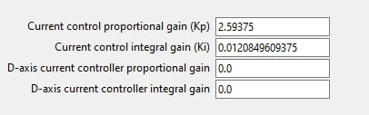 Current control parameters
- Current control proportional gain (Kp) (0x4641,13): Proportional gain for Q-axis current. It’s used to control the Iq currrent into the Target Iq.
- Current control integral gain (Ki) (0x4641,15): Integral gain for Q-axis current.
- D-axis current controller proportional gain (0x4641,33): Propotional gain for D-axis currrent. If set to 0, it will use the Kp value of the Q-axis.
- D-axis current controller integral gain (0x4641,34): Integral gain for D-axis current. If set to 0, it will use the Ki value of the Q-axis.
Modulation Index
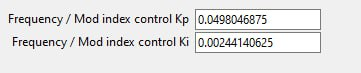
- Frequency / Mod index control Kp (0x4641,25): TO-DO
- Frequency / Mod index control Ki (0x4641,26): TO-DO
Speed Control
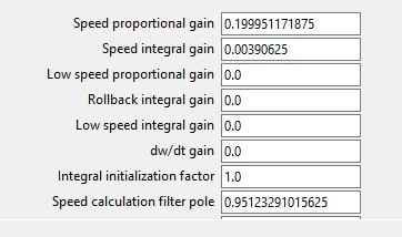
- Speed proportional gain (0x4651,1): Propotional gain to control speed. If we set a speed limit and this limit is achieved, inveter will use this value as proportinal gain to control the current to achieve that set speed.
- Speed integral gain (0x4651,2): Integral gain to control speed.
- Low speed proportional gain (0x4651,3): Proportional gain to control speeds on low RPM. This speed is configured on 0x4650,1 address and it can be 50 or 200rpm.
- Low speed integral gain (0x4651,4): Integral gain to control speeds on low RPM.
- Rollback integral gain (0x4651,5): Unused for our application.
- dw/dt gain (0x4651,6): TO-DO
- Integral initialization factor (0x4651,7): TO-DO
- Speed calculation filter pole (0x4651,8): TO-DO
Behavior Parametrization
These are parameters related to the vehicle’s performance or those that limit it without reaching the established safety maximums. There are 3 drive profiles and one baseline profile. If driveability have lower values than baseline, they will limit it. If baseline has a lower value, driveability will not un-limit it.
We can distinguish the following:
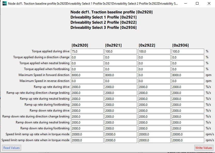 DVT driveability profiles
- Torque applied during drive (%) (0x2920,1): Percentage of torque applied during normal operation.
- Torque applied during a direction change (%) (0x2920,2): Unused as we don’t have steering sensor.
- Torque applied when neutral braking (%) (0x2920,3): Percentage of torque applied when vehicle is in neutral braking. Neutral braking means that FS1 switch is ON and throttle is 0.
- Torque applied when footbraking (%) (0x2920,4): Percentage of torque applied when footbraking is ON. You can configure footbrake as an input.
- Maximum speed in forward direction (rpm) (0x2920,5): Set a maximum motor RPM.
- Maximum speed in reverse direction (rpm) (0x2920,6): Not used for our application.
- Ramp up rate during drive (%/s) (0x2920,7): Defines the acceleration ramp, i.e. how fast or slow it will react to a torque request. It is important to set the highest value possible for this parameter to obtain a fast response on the accelerator.
- Ramp up rate during direction change braking (%/s) (0x2920,8): Unused as we dont have steering sensor.
- Ramp up rate during neutral braking (%/s) (0x2920,9): Acceleration ramp when vehicle is in neutral braking.
- Ramp up rate during footbraking (%/s) (0x2920,10): Acceleration ramp when vehicle is footbraking.
- Ramp down rate during drive (%/s) (0x2920,11): Defines the response ramp for when the throttle is released. I recommend entering a high value because if we enter a low value, we will see a slow response when we release the throttle and the bike continues to accelerate for a short amount of time.
- Ramp down rate during direction change braking (%/s) (0x2920,12): Unused as we dont have steering sensor.
- Ramp down rate during neutral braking (%/s) (0x2920,13): Deceleration ramp when vehicle is in neutral braking.
- Ramp down rate during footbraking (%/s) (0x2920,14): Deceleration ramp when vehicle is footbraking.
- Speed limit ramp up rate when in torque mode (rpm/s) (0x2920,15): TO-DO
- Speed limit ramp down rate when in torque mode (rpm/s) (0x2920,16): TO-DO
Safety Parametrization
These parameters are related to the safety of the vehicle, whether it is the battery, the engine or other elements. You have to be careful because these types of parameters limit the entire behavior of the inverter and sometimes we cannot realize it. For example, if we limit the maximum current of the battery for safety, it is possible that the inverter will never deliver the necessary amps to the motor and we will not obtain the desired torque.
Likewise, we can configure the maximum temperature of the motor and a cut-off table in which we define some gains. These will be applied progressively as the temperature is reached in the motor, so that the inverter will automatically cut the applied torque, preventing it from heating up even more.
Motor Limits
The motor limits are as follows:
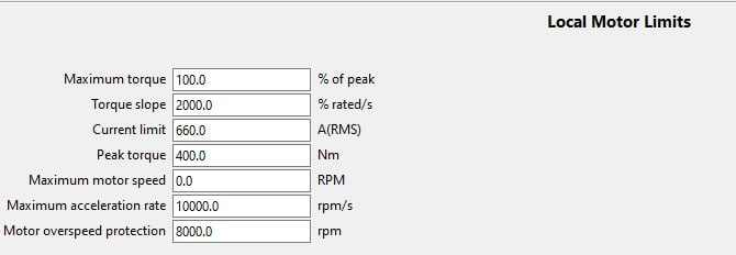 DVT motor limits
- Maximum torque (%) (0x6072,0): Maximum torque based on peak.
- Torque slope (%/s) (0x6087,0): Maximum rate of change of the torque. Set this on a high value to avoid slow torque appling.
- Current limit (A) (0x6075,0): Motor current limit.
- Peak torque (Nm) (0x6076,0): Motor peak torque.
- Maximum motor speed (rpm) (0x6080,0).
- Maximum acceleration rate (rpm/s) (0x6083,0): Set this parameter with a high value. If it’s low, motor will accelerate slow.
- Motor overspeed protection (rpm) (0x4624,0): RPM at which the inverter will trigger a fault.
Motor Thermistor
As we know, one of the limitations of an electric motor is the temperature it can reach. Motors have a temperature sensor embedded in the stator coils that is connected to the inverter, so the inverter knows the temperature of the motor at all times. There are several types of sensors such as KTY84 or KTY83. In general, it is quite standardized, so we can configure it in the inverter. In case the sensor is not defined, we have the option of creating a table in which we relate the temperature that the sensor should read with the reading resistance.
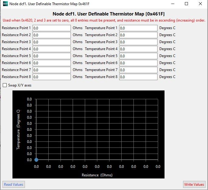 DVT temperature sensor map
Likewise, we can configure the maximum temperature of the motor and a cut-off table in which we define some gains. These will be applied progressively as the temperature is reached in the motor, so that the inverter will automatically cut the applied torque, preventing it from heating up even more.
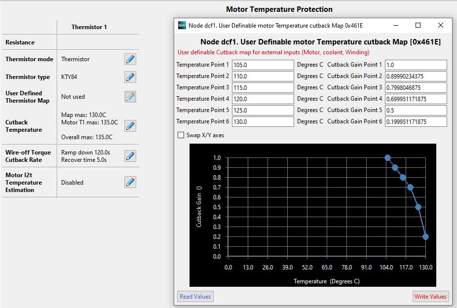 I2t configuration
We can also configure what we want to happen in case there is a cut or disconnection in the engine temperature sensor. The inverter has a temperature estimation option (i2t) if not PTC is present, which we will not use.
Battery Limits
In this section we are going to configure the voltages at which we want the inverter to begin to reduce the torque applied to the engine. In it we should define the maximum and minimum voltage that our battery supports and gradually cut off the applied torque. To do this we have a table with two values, the voltage and the cut-off gain. A 1.0 means that we will continue to deliver 100% of the torque, a 0.5 gain means that we will limit it to 50% and a 0.0 means that we will not deliver any torque, so the vehicle will stop.
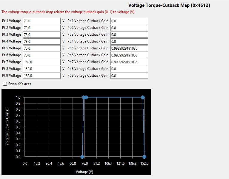 Battery gains
Advanced Settings
TO-DO
Encoder Alignment
TO-DO
Control Algorithms
As we mentioned before, Sevcon supports IPM and SPM engines. We have two algorithms for the engine, the Geometric and the lookup tables.
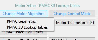 Control algorithm
PMAC Geometric
This algorithm is used for SPM engines. In this case, only the field weakening strategy will be applied.
PMAC 3D Lookup Tables
This algorithm is used for IPM engines and will apply the field weakening strategy and the MTPA. Both strategies will be implemented in the lookup tables.
Generating our own 3D Lookup Tables
TO-DO
Software Monitoring
After working with the DVT software for some time, it became clear to me that it doesn’t have enough tools for comfortably monitoring the inverter. The software primarily offers these three elements:
- Live vehicle interface: Real-time monitoring of inverter values is available, but it displays data in a table with small bars, which isn’t very user-friendly.
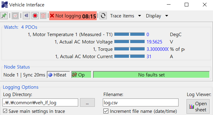 DVT log viewer
- Log Viewer: This feature generates an Excel file with charts for all the data. However, as shown, it’s not visually appealing or easy to navigate.
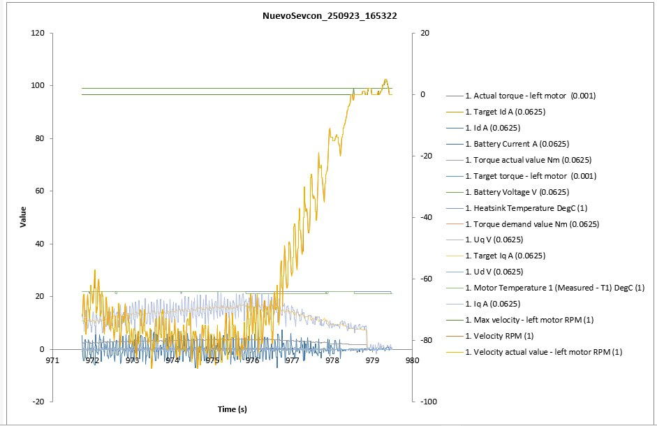 DVT output excel file
- Current control and field weakening: This graph shows the PI trace well, but it doesn’t support live viewing.
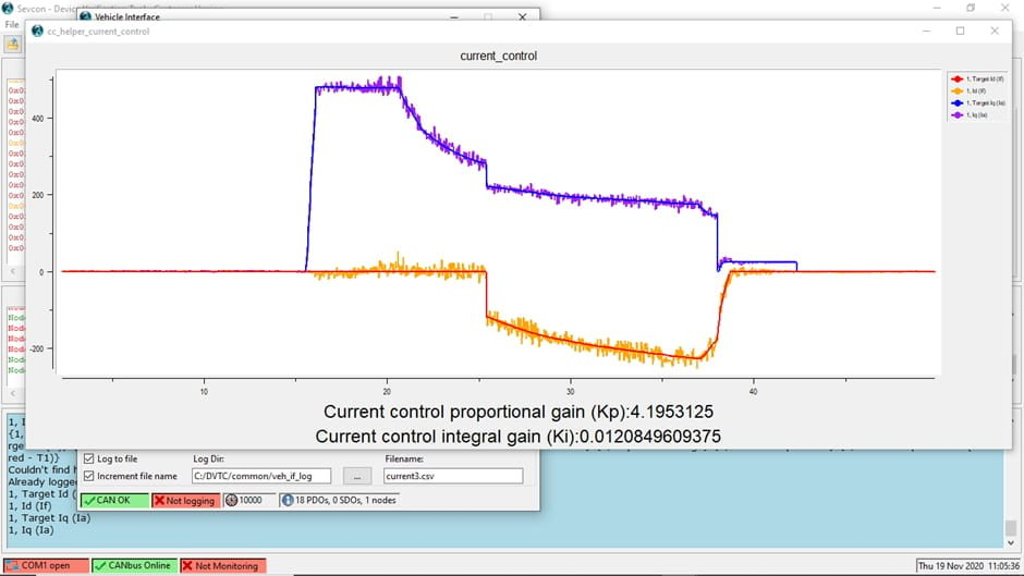 DVT current control monitor
I found none of these options practical or convenient, especially since we were planning to perform multiple dyno tests in rapid succession. So, I decided to develop custom software specifically for this purpose.
I chose to use Java (even though it’s not the ideal choice) because I was familiar with the JavaFX library, and libraries were also available for CAN interface connectivity.
I’ll likely publish the software in a few weeks, so I won’t go into development details here. However, here’s a preview of the software:
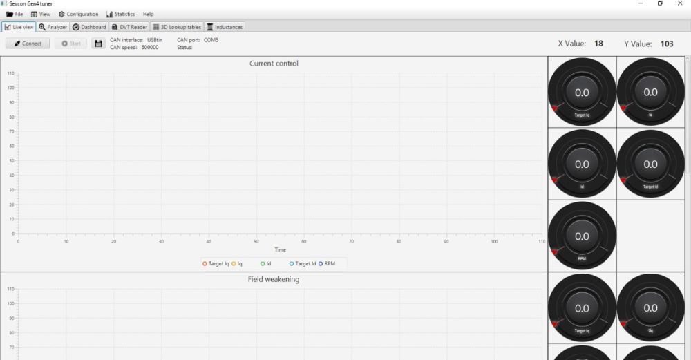 Live data plotter
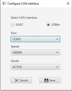 Interface configuration
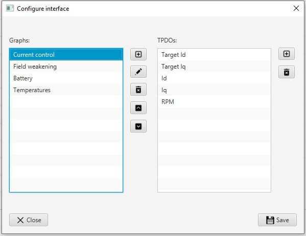 GUI configuration
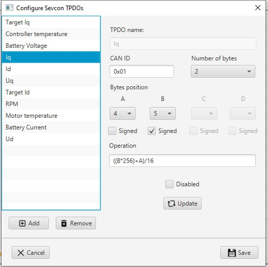 TPDO decoding
 Stats
Stats
 Log files
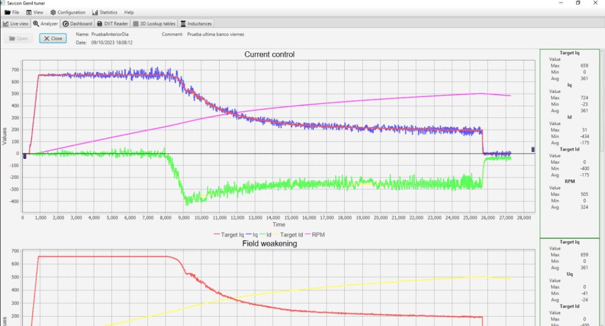 Analyzer
Dyno
I don’t have the latest graphs we got on the dyno but here is an example of one of them:
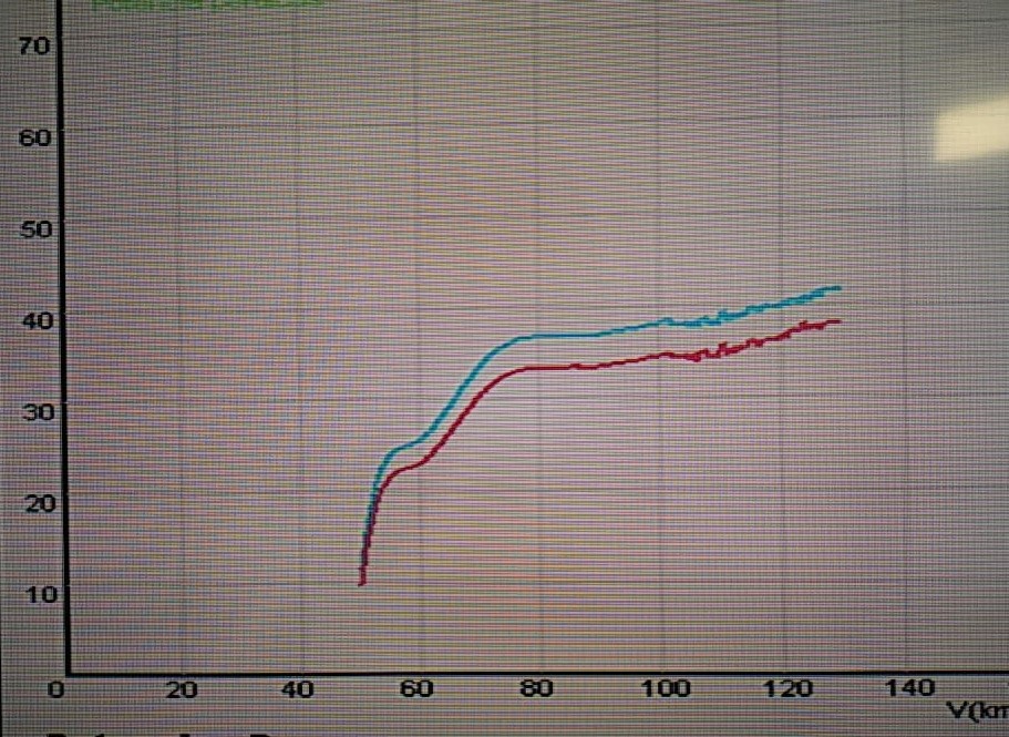 Dyno graph
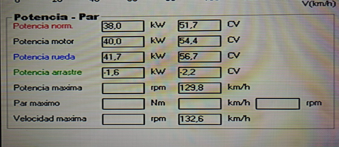 Dyno data
Results 📈
We achieved first position in the braking test, being the team that stopped the bike from 80 km/h in the least meters. Perhaps some important factors were the wheelbase of the bike and the size of the front brake disc. However, things don’t always go as expected. Despite the immense amount of work, the results on the other tests were not as expected. Although the bike operated without issues and everything worked as planned, we analyzed the results to identify areas for improvement. To do it, we reviewed official data from the event. Here are some conclusions we drew:
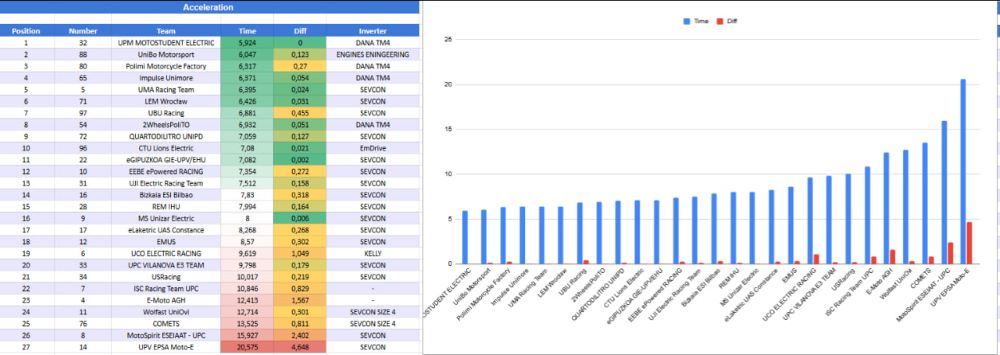 Acceleration test results
In the acceleration test, we placed seventh. We had two attempts: in the first one, we used a smaller crown and lookup tables on the inverter. In the second one, we could have used a larger crown for better results, but we were unsure if the motor would reach maximum revolutions, so we opted for a slightly smaller one.
Additionally, the top positions were held by bikes with Dana TM4 inverters, likely because these inverters support 750A, whereas the Sevcon is limited to 660A. The optimal setup might have been to use the Dana for the acceleration test and the Sevcon for the race. Even so, we were the third team in the acceleration test using Sevcon.
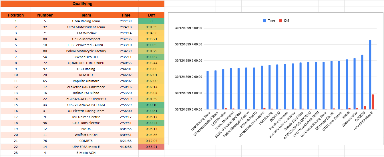 Qualifying results
In qualifying, our results were less competitive, and we couldn’t understand why. We noticed an anomaly in the telemetry data, which led us to question its accuracy. After verifying the code, we confirmed that everything was correct. The problem wasn’t technical as we are going to analyze later.
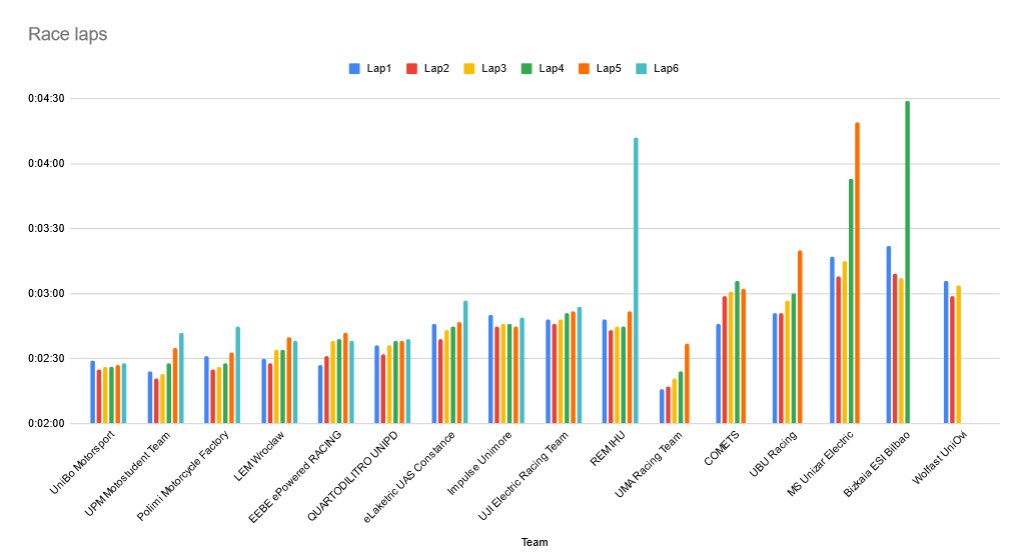 Race time by lap
The winning team stood out for its consistency. The UMA Racing Team was leading but encountered a disconnection in their motor temperature sensor, causing it to burn out. Meanwhile, UPM started strong but gradually lost performance, as seen from lap 5 onward.
Our driver took an incorrect line in lap 4 (yes, surprisingly), allowing UMA to overtake us, which caused us to complete one fewer lap. I don’t intend to blame anyone for the results but rather to highlight the mistakes made on all fronts. Technically, we identified the following areas for improvement:
- Battery too big: As we have said, due to the lack of telemetry in previous years and the early decision without correct inverter programming, we made a battery too big and heavy for the race.
- Fairing too big: The battery’s size needed a larger fairing, which negatively impacted the prototype’s aerodynamics.
- Large radiator: We mistakenly believed a larger radiator would provide better cooling, but the electric motor wasn’t able to transfer heat efficiently to the water. Therefore, cooling the water did not result in better motor cooling. This caused two issues: additional weight from the larger cooling circuit and increased aerodynamic drag from the radiator.
- Optimization of the mechanical parts: Some parts could have been optimized to reduce weight.
- Inverter programming: We initially set the motor to full power and reduced torque when it got hot. However, the optimal strategy would have been to gradually apply torque to balance temperature and maintain consistent torque.
Our biggest mistake was selecting a rider based on an assumption of experience, which turned out to be less competitive than expected. Here’s some data from the telemetry:
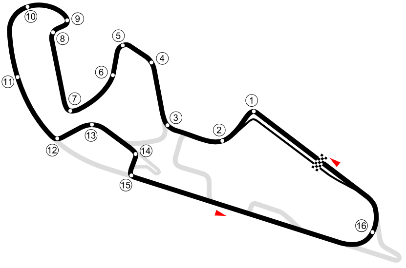 Circuit map
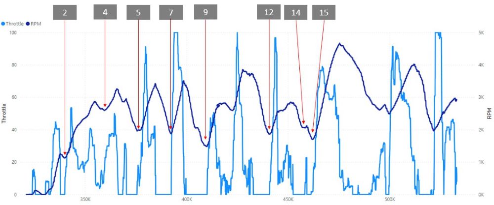 Telemetry
The graphs display throttle position and bike speed (direct transmission, so motor speed data is enough). Although we didn’t complete the GPS data module, each marked turn is visible, with the first lap showing the exit from the pits.
On the long straight starting from turn 15, speed increases gradually, yet the throttle isn’t fully open. The same pattern is evident at the next peak, the main straight. While this could be attributed to it being the first lap, we see similar behavior in later laps:
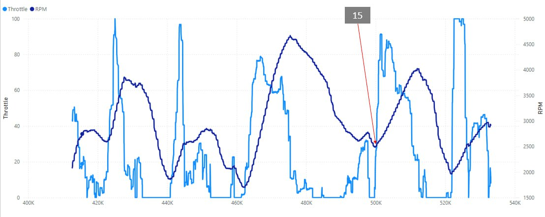 Telemetry data
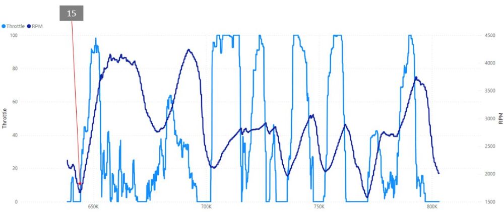 Telemetry data
In all of them, the throttle isn’t maintained at 100% until braking, it’s gradually released. It reaches 100% only on short straights. Also, speed on the straight after turn 15 increases slowly after the throttle is released. Examining the track’s altitude profile, this section is downhill.
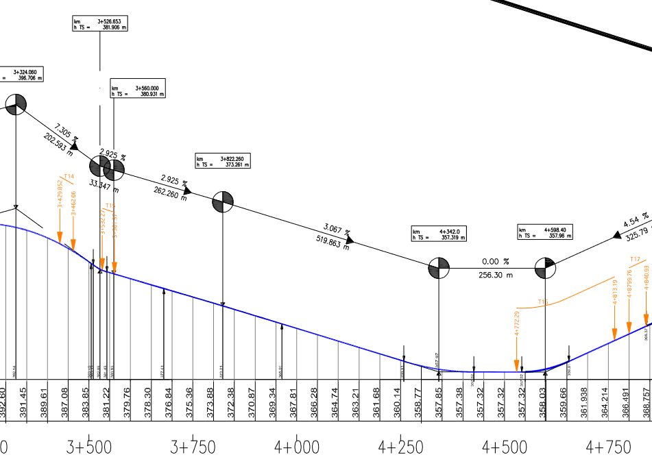 Circuit elevation profile
Our conclusion is that the driver was likely apprehensive about high speeds or the large circuit. We may never know for sure, but the data doesn’t lie. All these factors likely contributed to our lower than expected results.
We wanted to give a small gift to the sponsors who had supported the project when it ended and for this I made some 3D printed models of the prototype. To do this, with the 3D model of the prototype, I printed some models in SLA and cut some wooden boards that we engrave ourselves with laser.
Gallery 📷
References: