Building a Dynamometer from Scratch
Check out the project here: GitHub Repo
Introduction
After the previous project, my goal was to learn more about inverter programming for electric motors. I had the motor, inverter, and battery already available, but a proper way to test the system was still needed. Testing a motor and inverter dynamically (on a moving vehicle) is nearly impossible, as it requires a good data acquisition system and then dumping the data by connecting a cable to it. Doing this every time a parameter is changed would make the testing process inefficient and slow. Of course, a remote wireless monitoring system could be developed, but it is still not the best solution for controlled testing.
During the electric motorbike project, a company allowed the team to test the motorbike on their dyno, but that dynamometer was too large and heavy for practical and frequent use. Also, the electric motorbike project was closed due to the lack of university students committed to the project. This raised a simple question: why not develop my custom dynamometer?
Project Goal
The objective of this project is to design and build a custom dynamometer that serves two primary functions:
-
Performance Measurement: Understanding how specific inverter parameters affect behavior, torque, speed, and power output.
-
Thermal and Load Simulation: Analyzing the system’s behavior under stress. This involves studying how peak loads and continuous use impact the thermal behavior of the motor and electronics.
While professional electronics and dynos are available on the market, I took this as a multidisciplinary engineering challenge. Developing the system from scratch provided an opportunity to again integrate mechanical design, power electronics, and programming into a single functional tool.
Types of Dynamometers based on Absorption Type
Depending on the application and the complexity, different types of dynamometers can be found. Next, some of them are analyzed.
Inertia / Flywheel Dynamometers
 Inertia Dynamometer
 Inertia Dynamometer
This type of dynamometer is the simplest. It uses a large rotating mass (flywheel). The engine or motor accelerates the flywheel and performance is measured based on how quickly the flywheel speed increases. In this type of dynamometer, no active braking system is used. The test ends when the system stops accelerating at maximum speed.
Advantages:
- Simplicity and cost: The mechanical design is simple, making it the most affordable entry point for power measurement.
- Simulates acceleration well: It provides a good representation of acceleration performance.
- Low maintenance: No friction parts need replacement, and no complex cooling systems are required, as energy is stored kinetically rather than dissipated as heat.
Disadvantages:
- No Steady-State Testing: It cannot hold a motor at a specific RPM (for example, 3000 RPM at 50% throttle) to tune maps or other parameters.
- Limited control over load.
- Safety design at high speeds: Measuring a high-power motor requires a large flywheel, which can be achieved with either a heavy mass or a larger diameter with less mass. Care must be taken with the forces experienced by the flywheel at high speeds.
Friction / Mechanical Dynamometer
 Friction Dynamometer1
This type of dynamometer uses friction (brake discs like in cars, belts, or a Prony brake) to provide load. Torque is measured from the reaction arm with a load cell.
Advantages:
- Simple, low-cost design.
- Easy to build and maintain.
Disadvantages:
- Low precision.
- Limited repeatability and control.
- Generates significant heat making it unsuitable for continuous operation.
Water Dynamometers
 Water Dynamometer
 Water Dynamometer
 Water Dynamometer
This type of dynamometer uses water as a resistive medium. It has rotating impellers that push against water, and torque is absorbed as hydraulic resistance. Torque is measured with a load cell connected to a reaction arm on the housing.
Advantages:
- High torque capacity, suitable for heavy-duty applications.
- Simple and robust design.
Disadvantages:
- Requires a continuous water supply and cooling system (on a closed tank).
- Expensive if you have to build your own.
Hydraulic Dynamometers
 Hydraulic Dynamometer2
Similar to a water brake, but uses hydraulic fluid instead of water. Some designs are more compact and efficient.
Advantages:
- Compact design.
- Can handle medium to high power levels.
Disadvantages:
- Requires careful cooling and regular oil maintenance.
- More complex than simple water brakes.
- Pumps tend to work only at low RPMs (depending on the pump).
Motor Generator Set
 Motor GenSet
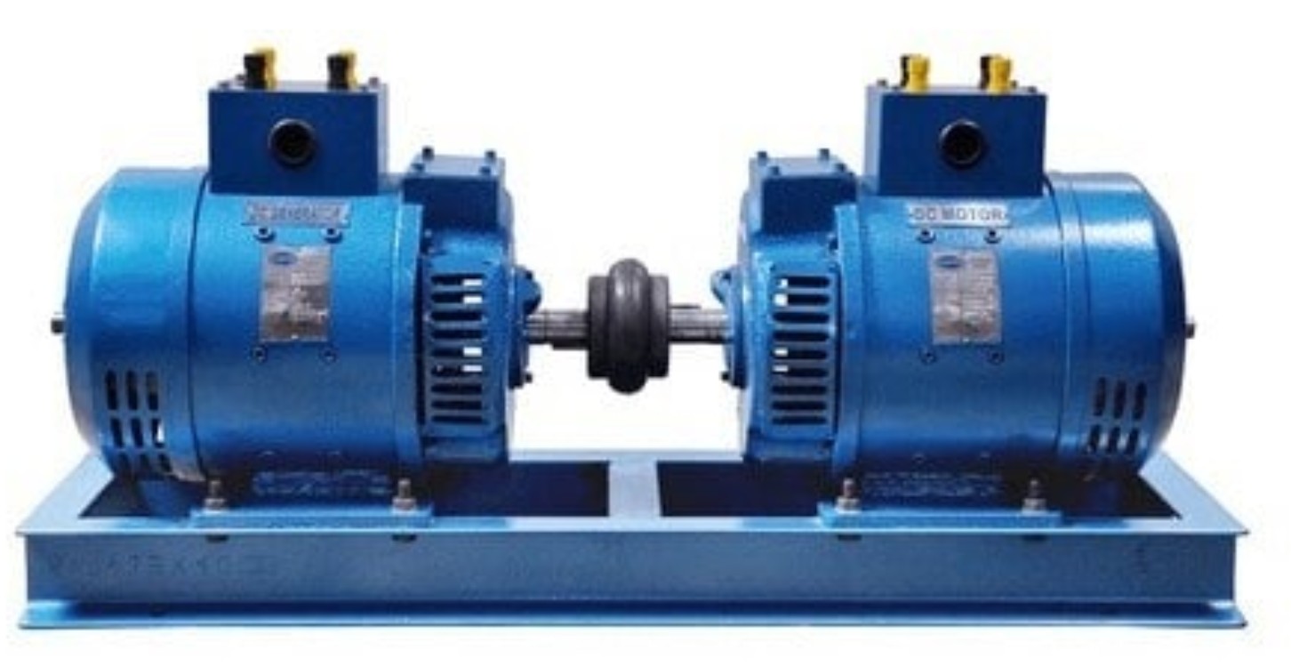
A motor-generator set uses one motor to drive another motor or generator which acts as a load. The system can convert mechanical energy back into electrical energy, which can then be reused or dissipated. This type of dynamometer is useful for testing motors while minimizing energy losses.
Advantages:
- Low power consumption: As the DC links are connected between the machines, the only losses come from system inefficiencies (heat, friction, and electrical losses).
- High precision: Can simulate various load conditions accurately.
- Regenerative capabilities: Energy can be fed back into the supply, reducing operating costs for long tests.
Disadvantages:
- Requires two matched motors and ideally inverters: Both machines must achieve the same maximum speed and torque characteristics.
- More complex control and setup compared to simpler dynamometers.
- Larger footprint and higher initial cost.
Eddy Current Dynamometers
 Roller Eddy Current Dynamometer
 Eddy Current Dynamometer
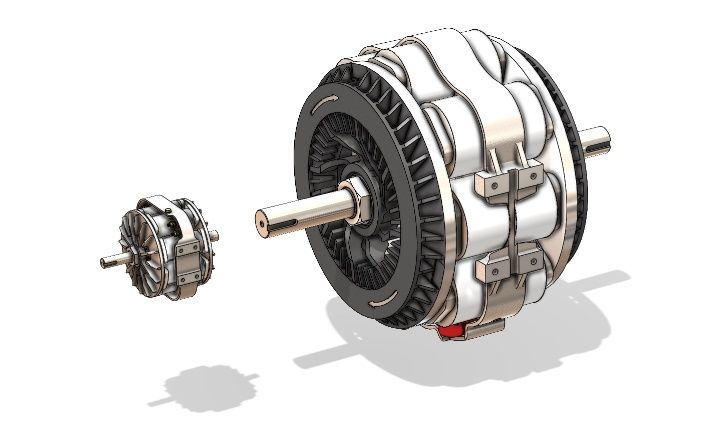
Eddy current dynamometers use electromagnetic induction to create a braking force. The rotor spins inside a strong magnetic field, generating eddy currents in the rotor, which produce resistance proportional to the current applied. Torque is measured using a load cell, and the system can be precisely controlled electronically.
Advantages:
- Precise load control: Easily adjustable for different torque and power conditions.
- Fast response: Ideal for transient and dynamic testing.
- Compact and low maintenance: No direct mechanical friction, reducing wear.
- High repeatability: Allows consistent testing for calibration and performance analysis.
Disadvantages:
- Limited effectiveness at very low speeds, as some rotor motion is required to induce braking.
- Generates heat that must be managed with air or water cooling.
- More expensive than simple mechanical or hydraulic dynos.
Table Comparison
| Type | Principle | Advantages | Disadvantages |
| Inertia / Flywheel | Acceleration of a known rotating mass | Simple, inexpensive, no active load system, low maintenance | No steady-state capability, no load control, safety concerns at high speed |
| Friction / Mechanical | Mechanical friction | Very simple, low cost, easy to implement | Low accuracy, poor repeatability, high heat generation, wear |
| Water Brake (Hydraulic) | Hydrodynamic resistance using water | Very high torque capacity, robust, suitable for continuous operation | Requires water system, slower response, less precise control |
| Hydraulic (Oil) | Hydrodynamic resistance using oil | Compact, higher efficiency than water systems, good load capacity | Cooling and fluid maintenance required, more complex system |
| Electric (Motor/Generator) | Electromechanical energy conversion | High precision, four-quadrant operation, regenerative energy recovery, full control at all speeds | High cost, complex control and infrastructure |
| Eddy Current | Electromagnetic induction | Fast response, precise load control, low maintenance, good repeatability | Torque proportional to speed (ineffective at very low RPM), requires cooling |
Types of Dynamometers Based on Interface Type
Aside from the absorption method, dynamometers can also be classified by how they interface with the motor or vehicle. The four main types are engine dynos, hub dynos, roller dynos and vehicle dynos.
Engine Dynamometer
 Engine Dynamometer3
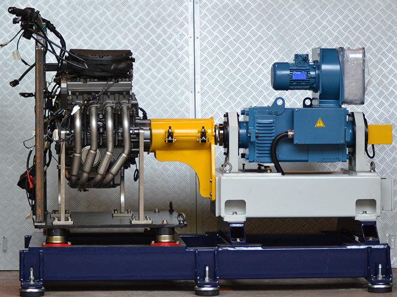
Engine dynamometers couple the motor or engine shaft directly to the absorber through a coupling or driveline. Because there is no drivetrain loss or tire slip involved, they provide the most accurate torque and power measurements. This makes them the preferred choice for motor and engine development, mapping, and calibration.
Eddy current brakes, water brakes, and motor-generator sets are all commonly used as the absorption unit in this configuration. Since the motor is isolated from the rest of the vehicle, these dynos are typically equipped with a large number of sensors to monitor both internal signals (coolant temperature, oil pressure, exhaust gas temperature) and external measurements (torque, speed, power, ambient conditions).
The main downside is that the motor must be removed from the vehicle and rigidly mounted to the test bench, which requires dedicated infrastructure and alignment work.
Hub Dynamometer
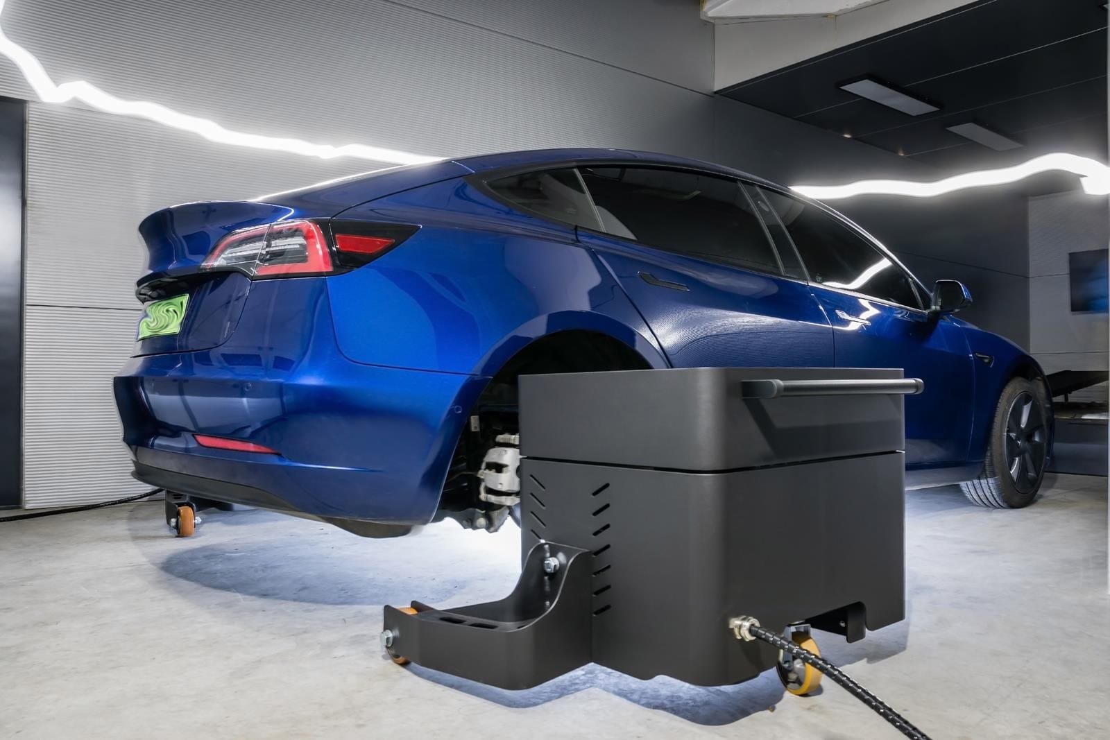 Hub Dynamometer
Hub dynamometers bolt directly to the wheel hubs of a vehicle, replacing the wheels entirely. This eliminates tire-to-roller slip losses (present in roller dynos) while still allowing the full drivetrain to remain in place. The result is a measurement accuracy that sits between engine dynos and roller dynos.
The main advantage is convenience: only the wheels need to be removed to set up the test. No engine extraction or rigid coupling alignment is needed, making it much faster to get a vehicle on the dyno. However, drivetrain losses (gearbox, differential, driveshaft) are still present in the measurement, so the values reflect power at the hubs rather than at the crank or motor shaft.
This type is popular in aftermarket tuning and motorsport, where quick turnaround times and repeatable results are more important than absolute crankshaft power figures.
Roller Dynamometer
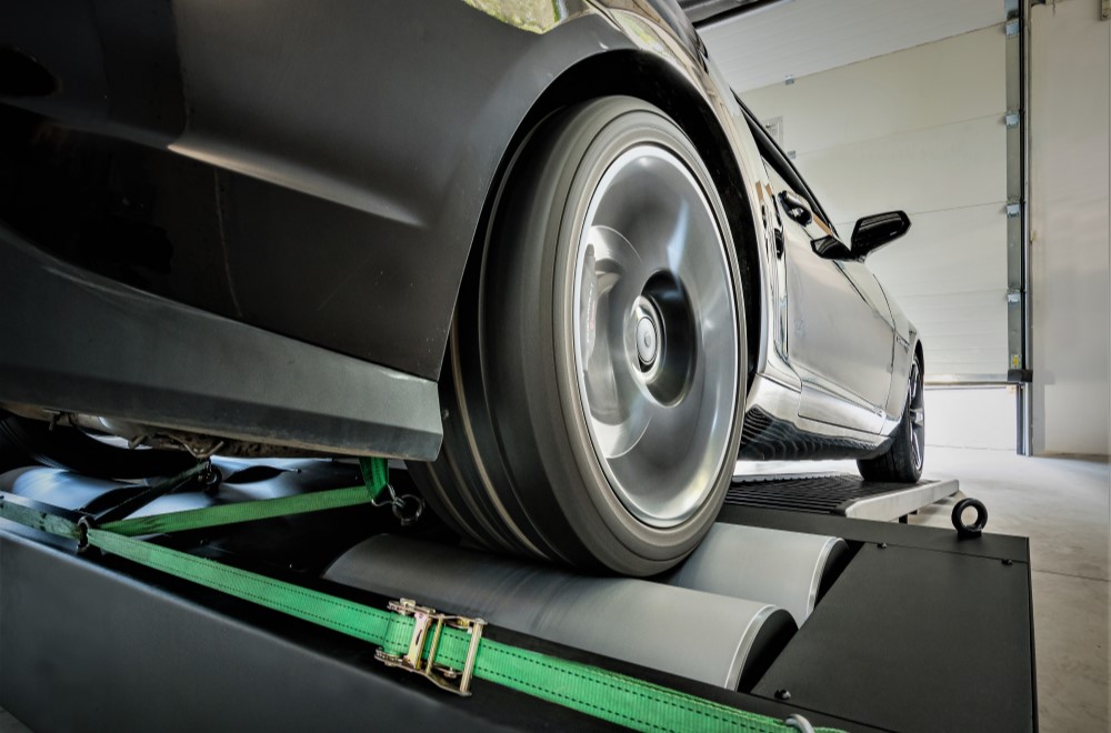 Roller Dynamometer
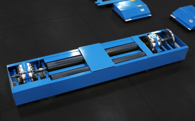
Probably the most well-known type, the roller dynamometer (or chassis dyno) places the entire vehicle on a set of rollers. The driven wheels sit on the rollers, and the vehicle accelerates them as it would on the road. The absorber unit is connected to the roller shaft, measuring the power transmitted through the tires.
They are the least accurate of the three types due to tire-to-roller friction and potential slippage, especially on high-torque vehicles. Well-designed roller dynos mitigate this by using two rollers per axle: one connected to the absorber for power measurement, and a free roller. Both rollers are equipped with encoders so the system can detect slip and correct or invalidate the test run accordingly.
Despite their lower accuracy, roller dynos are extremely popular because they require no vehicle modification at all. Drive on, strap the car down, and run the test. They are widely used in tuning shops, workshops, and performance diagnostics.
Vehicle Dynamometer
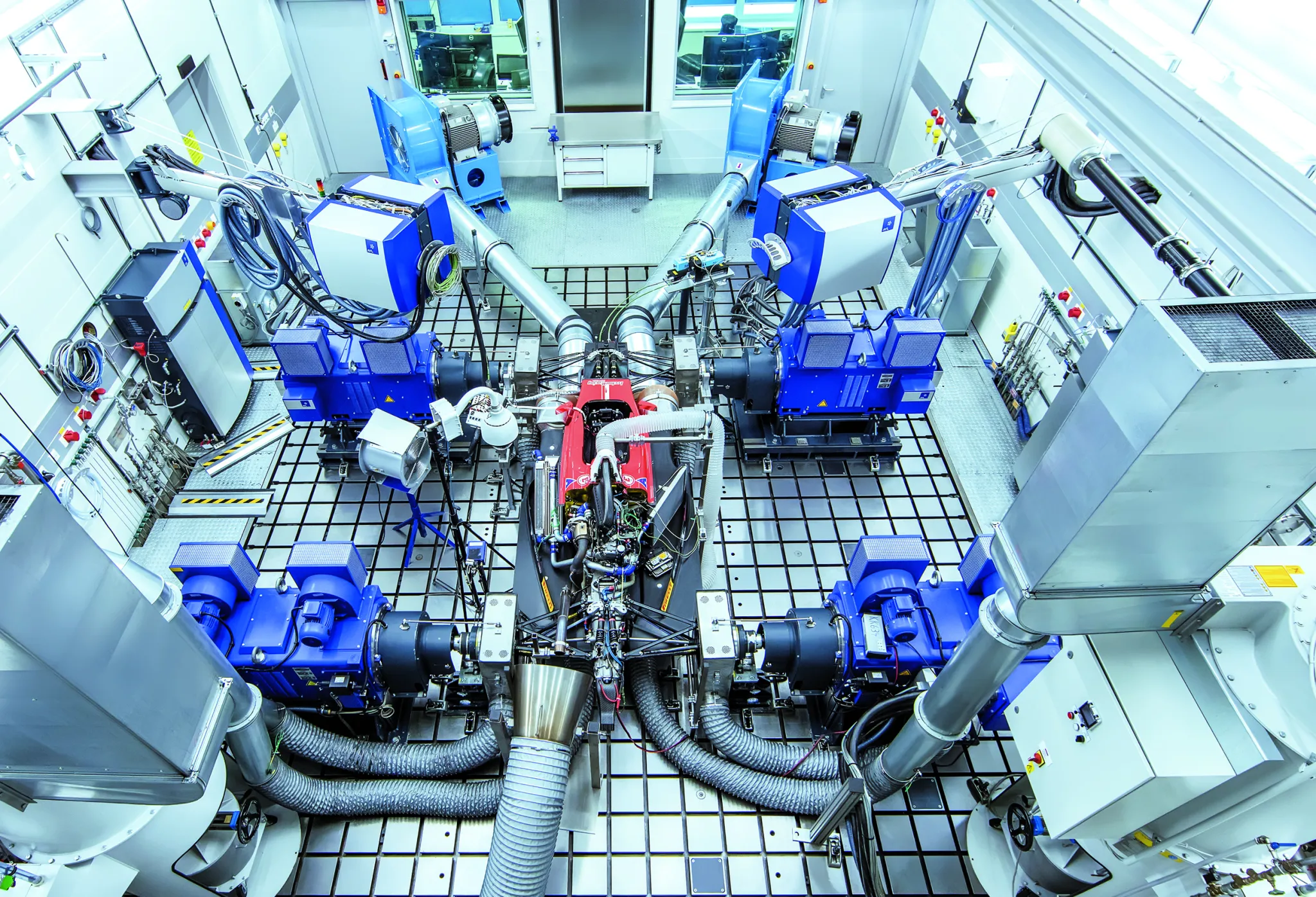 Vehicle Dynamometer
These are among the most advanced dynamometers available. The entire vehicle can be mounted on the system, which simulates real-world driving conditions and vehicle behavior. This type of dynamometer is used by top-tier motorsport organizations, including Formula 1 teams, for final testing and development work.
Initial Approach
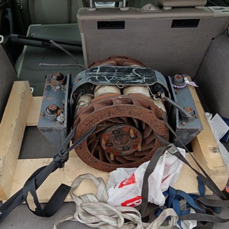
Based on my requirements, the two best options were an eddy current brake or a water dynamometer. While exploring a junkyard, I found a cheap (350 €) and relatively small (500 hp) eddy current brake. This quickly decided the choice. Water brakes are not as affordable as eddy current dynos, even on the second-hand market, and they require a water tank and sometimes a water cooler to operate, making them more complex and cumbersome for this project.
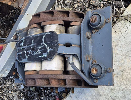 Junkyard Eddy Current Brake
Another important requirement was to supply the eddy current brake using a standard electrical socket (230 VAC in Europe). Using an external battery was not desirable due to the need for constant monitoring and recharging.
How Eddy Current Brake Works
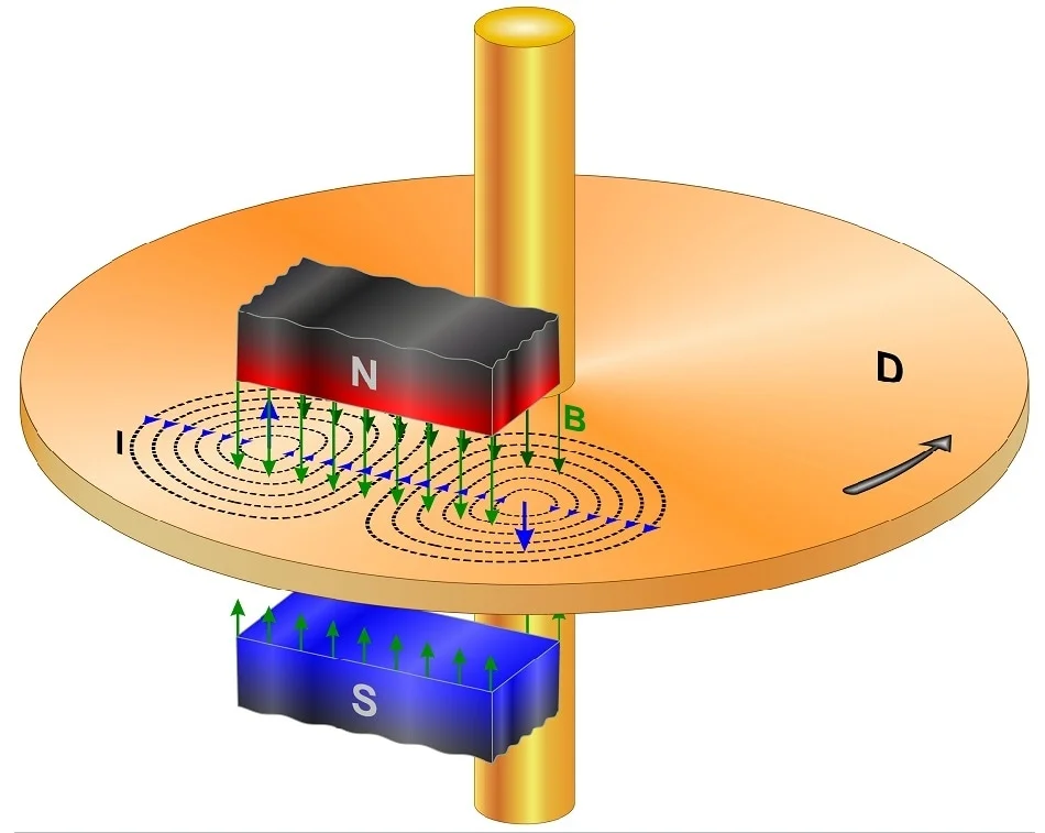
The first thing to understand is how an eddy current brake works. These brakes do not have any friction parts. They use electromagnetic force to create braking torque.
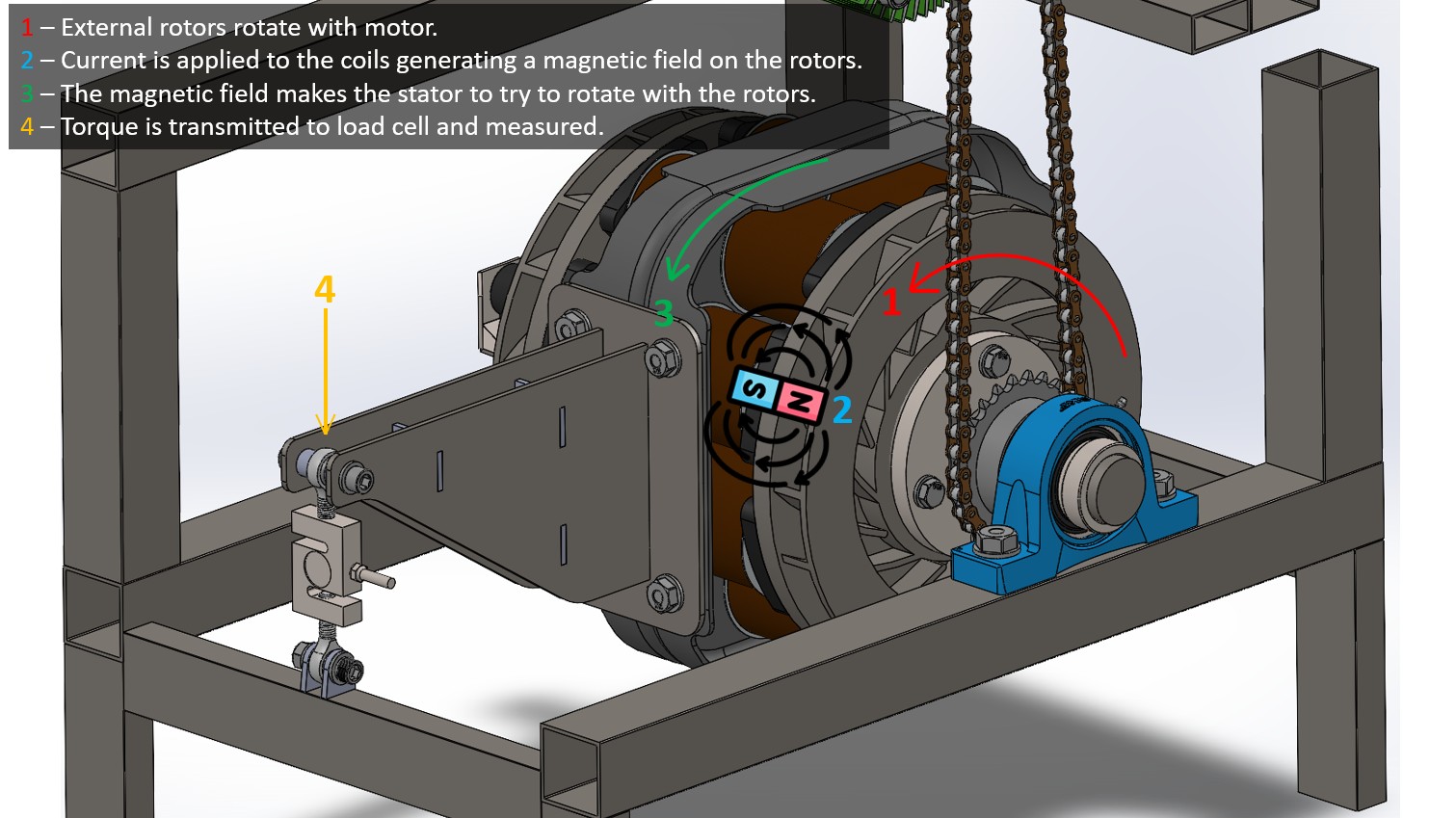
 Eddy Current Brake Operation
 Eddy Current Brake Operation
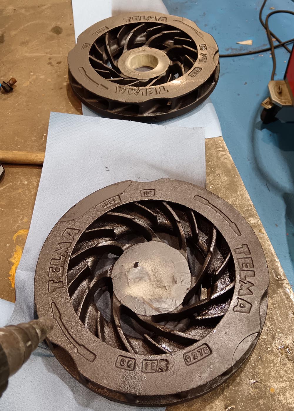
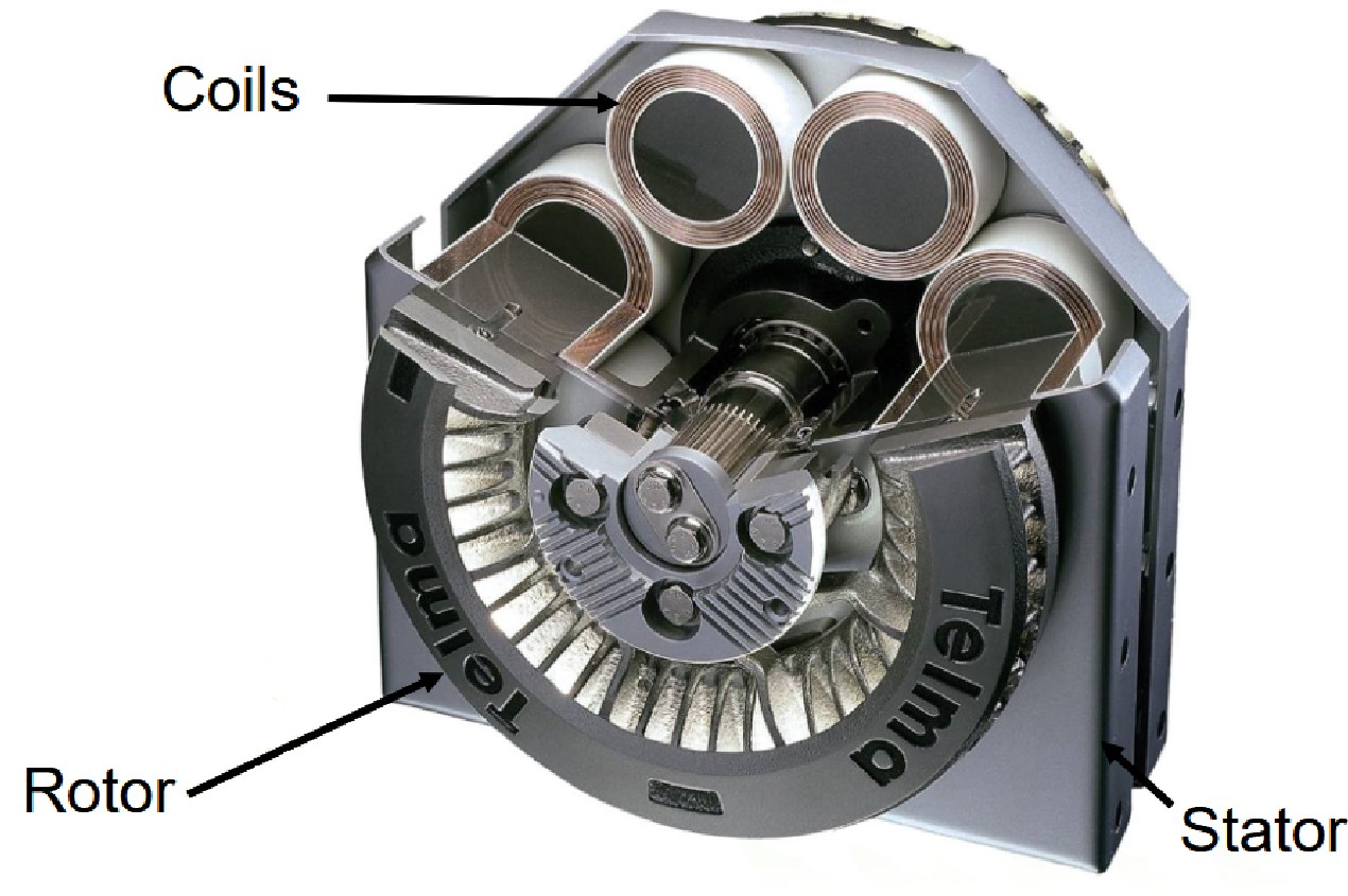 Eddy Current Brake Parts
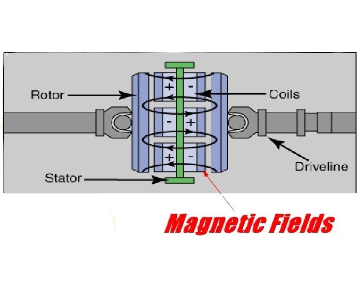
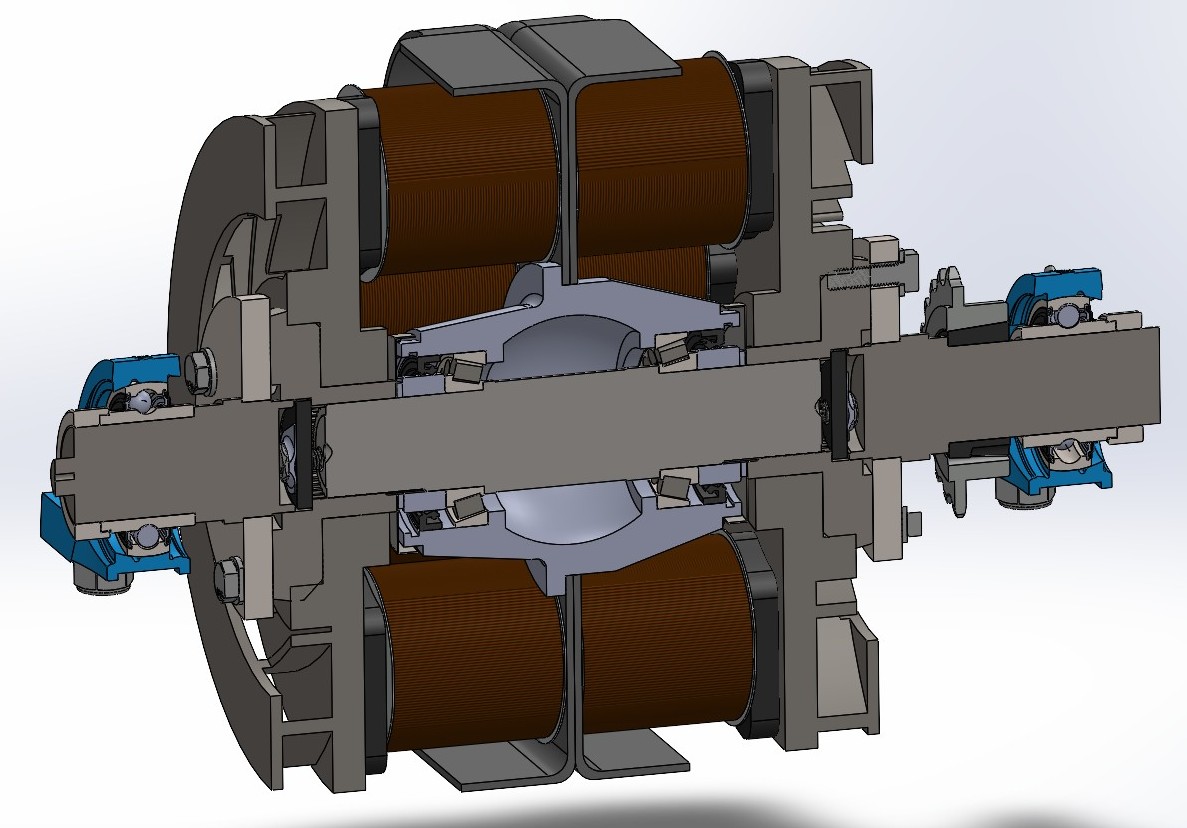
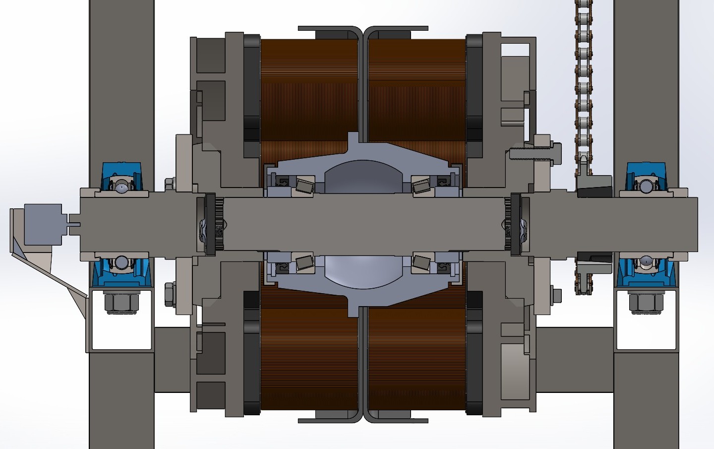
As shown in the images, these brakes have three main components:
- Rotor: Composed of two steel discs that rotate. The rotor is the moving part on which torque is applied.
- Stator: The static part of the brake which houses the coils.
- Coils: These generate the electromagnetic field that interacts with the rotor to produce braking torque.
When voltage is applied to the coils, a magnetic field is generated. As the rotor (lateral discs) spins through this magnetic field, eddy currents are induced in the steel rotors. According to Lenz’s law, these currents generate an opposing magnetic field that resists the motion of the rotor creating a smooth and controllable braking force.
The braking torque is proportional to the current applied to the coils and the rotor speed. At low speeds, the braking force is weaker, which is why eddy current brakes are less effective at very low RPMs. However, their fast response and precise control make them ideal for motor testing.
 Eddy Current Brake Working Principle
Eddy current brakes also generate heat in the rotors due to the induced currents. Proper cooling, either air or water, is necessary to maintain consistent performance during extended tests. This design allows for high repeatability, low maintenance, and accurate measurement of torque and power.
Another important point is that these brakes have an ideal structure for building a dynamometer. The stator is located at the center of the brake, making it possible to attach a load cell directly to it. The coils are housed in the stator and when braking torque is generated, the resulting force is transmitted to both the stator and the load cell.
The rotors are positioned on both sides of the brake which allows the brake to be held securely at these points (the shaft). This configuration also enables force to be applied from these points using a chain, a belt, or directly to the shaft via a cardan joint.
Here you have a great video from Telma on the original application of eddy current brakes, a truck retarder / electric brake that shows how it works:
In the case of a dynamometer, the weight of the eddy current brake is supported by the shaft instead of the housing, keeping the stator (the coils, or central part of the brake) “floating.” By attaching a load cell at a specific distance from the shaft, the torque produced by the brake can be measured accurately.
 Eddy Current Brake Working Principle
Project Overview
After having clear that I was going to use an eddy current brake I needed to plan all the system requirements. These initial requirements were:
- All the necessary mechanical components to hold the brake and the motor.
- All the electronics required to control the eddy current brake.
- All the software needed to control the system, allow user interaction and show test results.
Mechanical
- A structure to securely hold the eddy current brake.
- A motor holder to attach the motor to the brake.
Electronics
- A system to supply power to the eddy current brake.
- A system to manage the logic of the process, read signals and sensors, and perform fast calculations.
- A system to handle the user interface, allowing interaction with the logic system and access to data and output results.
Software
- Firmware to control all real-time signals and processes in the microcontroller.
- An application to allow the user to operate, control and monitor the system.
With this idea more or less clear I started with the mechanical design.
Mechanical ⚙️
The first thing I needed was an eddy current brake. I found a cheap one in the junkyard. There were multiple available but I was looking the smallest one as the electric motors I wanted to test were not very big.
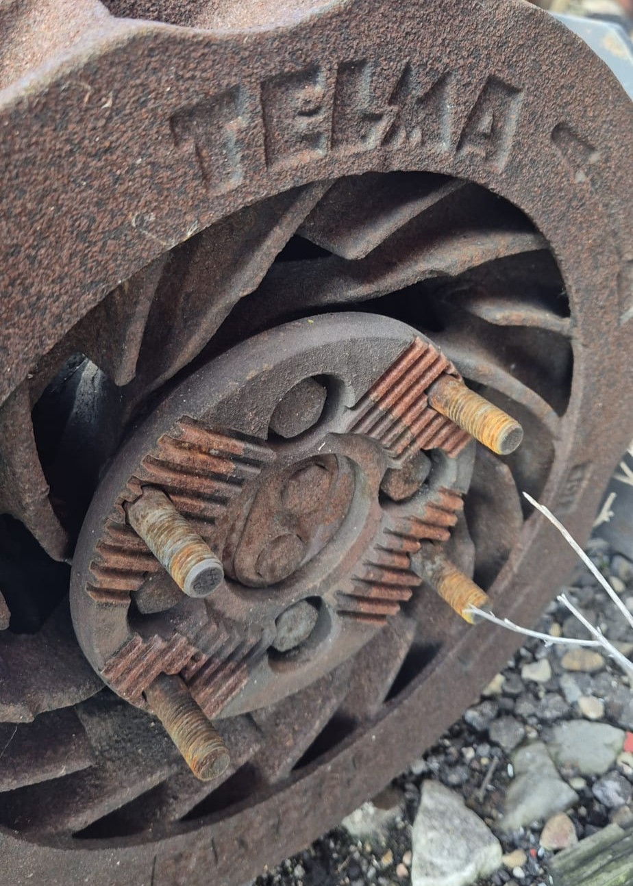
 Rusty Eddy Current Brake
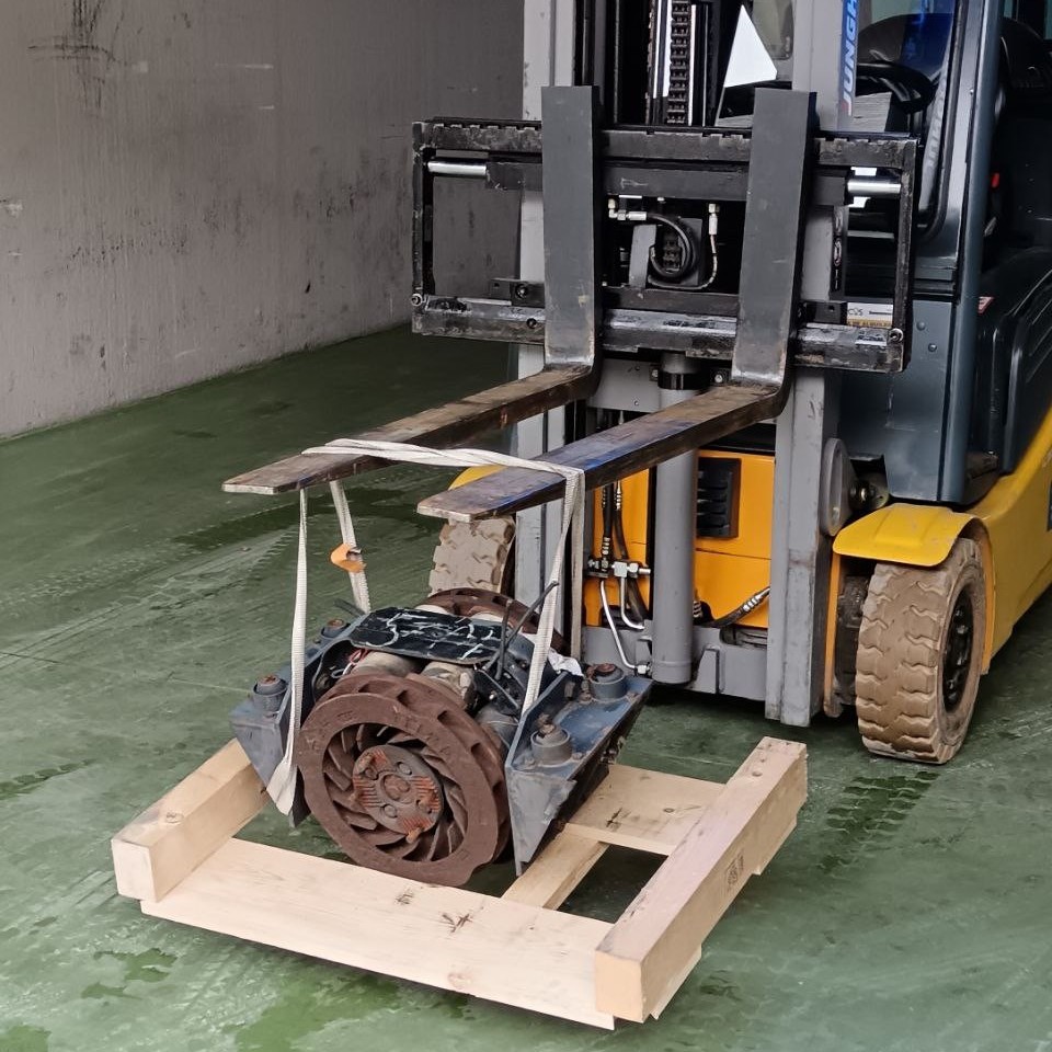 Rusty Eddy Current Brake
After cleaning and checking it, I found that it was a Telma AC 51 - 00. I sent an email to the company and fortunately they answered with the datasheet.
I needed to restore it a bit as it was on the street and a lot of parts were rusted and degraded.
 Rusty Eddy Current Brake
 Painted Rotors
Note that the rotors can achieve very high temperatures so special paint is needed.
Telma AC 51 - 00
This is a relatively small brake manufactured by Telma with a maximum torque brake of 1000 Nm and a bit more than 500 hp. For my project it was more than enough as I was going to brake a maximum of 140 Nm and near 40 HP peak.
Mechanical Characteristics of Eddy Current Brakes
The first thing we need to do is to analyze the characteristics of the eddy current brake we are going to use. This will set some characteristics of the system we are going to develop. Let’s focus on this eddy current brake, the Telma AC 51 - 00.
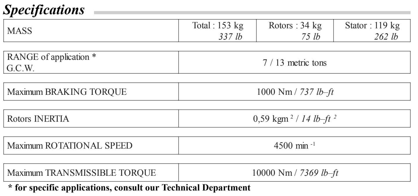 Telma Mechanical Specifications
In the table we can see three important characteristics of the brake:
- Rotors Inertia: This is the inertia of the rotors. We must add them to the torque calculation because when the system is accelerating, the torque/power required to accelerate this inertia will not be measured in the load cell.
- Maximum Braking Torque: This is the maximum torque the eddy current brake can hold. In this case, 1000 Nm, more than enough.
- Maximum Rotational Speed: This is the maximum speed at which the eddy current brake can rotate. This is a very important parameter.
I was going to test electric motors that can achieve 6000 RPM and 8000 RPM so I needed a reduction between the motors and the eddy current brake.
Another important characteristic of these brakes are the power and torque curves. Here we can see them:
 Telma Torque and Power Curves
As we can see, this brake has 4 control stages. This is based on the original use of the brake as a retarder. We are going to skip this now as we will analyze it later.
Mechanically speaking, we need to understand that this type of brake has losses. Some of these losses are reflected in the load cell so we don’t need to care about them but others we need:
- Brake torque produced by the eddy current: This will be “directly proportional” to the current applied to it. All this torque will be measured by the load cell.
- Brake torque produced by the bearing losses: The internal bearings will have small losses because of friction and adjustment but we will see these losses in the load cell too.
- Brake torque produced by the inertia acceleration: As mentioned previously, when accelerating the brake, part of the torque applied will be lost in the mass acceleration and not measured in the load cell. We must take care about this loss.
- Brake torque produced by the rotor fans: This is probably the most missed loss. As the brake spins faster, the rotors act also as big fans moving a huge mass of air. This air is used to cool itself but also creates a resistive torque that is not measured by the load cell.
I didn’t take into account this last brake loss as I only wanted comparative tests but several manufacturers don’t take it into account, and from my point of view it’s an important loss to measure. At high speeds and when the eddy current brake is big and has big fans, this loss is important.
Another important consideration is that eddy current brakes do not perform efficiently at low RPM. For high-power testing, a minimum of 500 RPM is typically required to reach the constant torque region and ensure stable braking. Applying high excitation current at very low RPM can cause torque ripple (cogging) and excessive heat soak. However, since I am measuring low-power motors, the required current will be low enough that these issues should not be a limiting factor.
Finally we need to take care about two more things. The first one is that the torque is not perfectly linear with the current applied. Depending on the RPM and the current applied the torque doesn’t follow a linear function. At low RPM they require a bit more current to generate the same torque than at higher RPM. I’m not going to worry about this now but if you need to build a perfect one, you need to take care about this to build a perfect control system.
It’s important to take care about the brake size when designing a dyno. Depending on the use we are going to do with it and the power of the motor that we are going to measure, we need to take care of the brake heating.
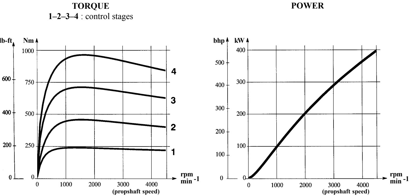
These brakes dissipate the energy in heat. This heat is produced on the rotors. As the rotors get hotter, the brake torque produced by them is lower. We can see it from another Telma datasheet here:
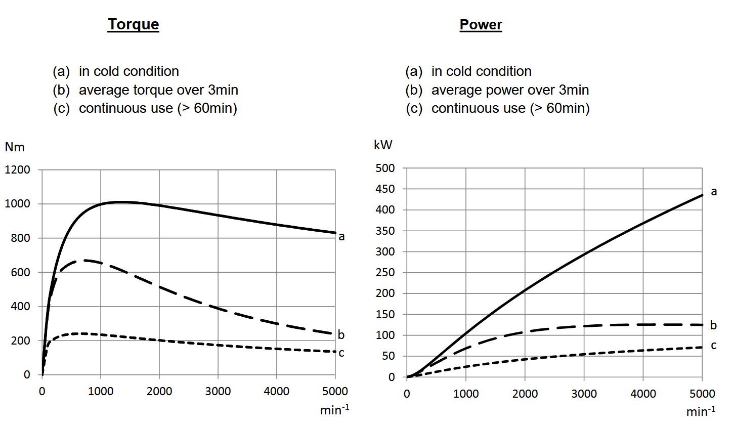 Thermal Losses
As you can see, as the eddy current brake is used and temperature increases, the available torque to brake drastically decreases. It also happens with the power. This means, as the heat increases in the rotors, the brake torque produced will decrease.
We can see in the graphs that when the eddy current brake is cold, this specific model is able to brake around 1000Nm and near 450Kw. As the temperature increases (because of the constant use), the available breaking torque drops drastically. This means that if for example we want to test continuously a motor or engine of near 100kw (134 hp), we will need to use a brake of around 450 kW (603 hp). Think about the use you are going to give to the brake. For example, in my case the runs were going to be of maximum 30 seconds and my limit was by far the electric motor so no problem for my application, but if you are going to brake a 500Hp engine for example and the tests will be long, you will need to think about a bigger eddy current brake or mounting two in series.
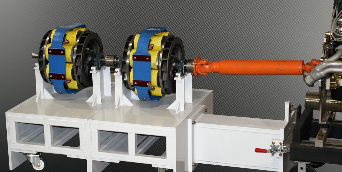 Dynamometer with two eddy current brakes
Cooling Considerations
As discussed previously, the rotors act as internal fans, pulling air through the brake housing to dissipate heat. For short acceleration runs like mine (under 30 seconds at relatively low power), this passive self-cooling is more than sufficient. The rotors heat up during the test but cool down naturally between runs. However, if you plan to brake higher power levels or run extended steady-state tests, passive cooling will not be enough. The rotors will continue to accumulate heat and, as shown in the thermal derating graphs, the available braking torque drops drastically as temperature increases. In those scenarios, an external forced-air cooling system becomes essential.
The simplest approach is to mount a high-flow industrial fan directly onto the brake housing, aligned with the existing air channels so it forces fresh air through the rotor gap. For even more demanding applications, some builders duct compressed air or install a dedicated blower.
Initial Adjustment
Before mounting the eddy current brake into the structure, I disassembled it and restored it as it was oxidized. The internal bearings were in acceptable condition. I cleaned everything and mounted it again.
When assembling these brakes we need to take care about two adjustments:
- Air Gap
- Bearing Adjustment
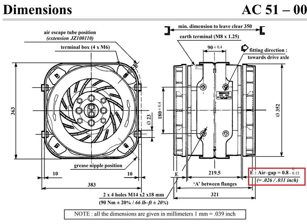 Telma Datasheet
As we can see here in the datasheet, the Air Gap (distance between rotors and coils) must be of around 0.8mm. If we assemble it closer it’s possible that the rotors rub against coils. If the distance is bigger the brake will lose efficiency and brake torque.
The bearing adjustment is used to fit the rotors with the housing/coils so all the structure keep rigid but not too much. The rotors must be able to rotate easily but also not being loose.
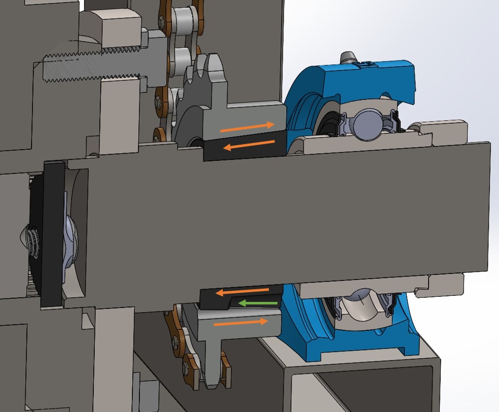
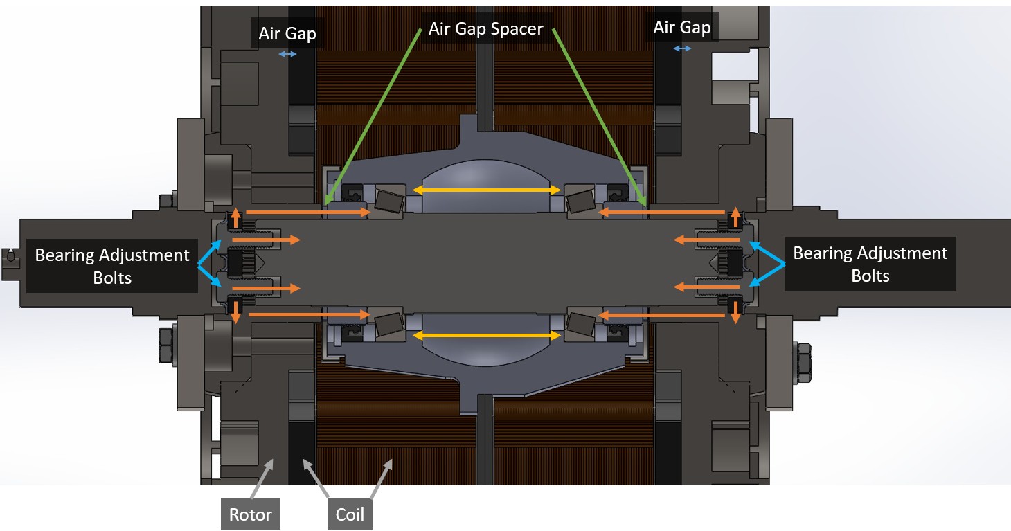 Eddy Current Brake Adjusters
Here we can see clearly both adjustments. The internal bearings are adjusted with the 4 bolts on both sides of the shaft. These bolts are not tightened fully so they have a clip to avoid losing them. If you follow the orange arrows you can see how this “packaging” works. The yellow arrows represent the internal spacer where the bearings are supported.
The air gap is adjusted changing very thin washers that are where the green arrows mark. If the washers are thinner, the rotors will be closer to the coils and if they are thicker the rotors will be further away from the coils.
After knowing all this information and adjusted these settings, I started drawing the brake on the CAD software.
CAD Design
With the brake ready I started designing the entire structure to hold both the unit and the motor. One of the most important factors was the speed limitation of the components. The maximum speed of this eddy current brake is 4500 RPM but I needed to rotate the motor up to 8000 RPM. For this reason I decided to use a chain drive with a reduction ratio to keep the brake within its safe operating range.
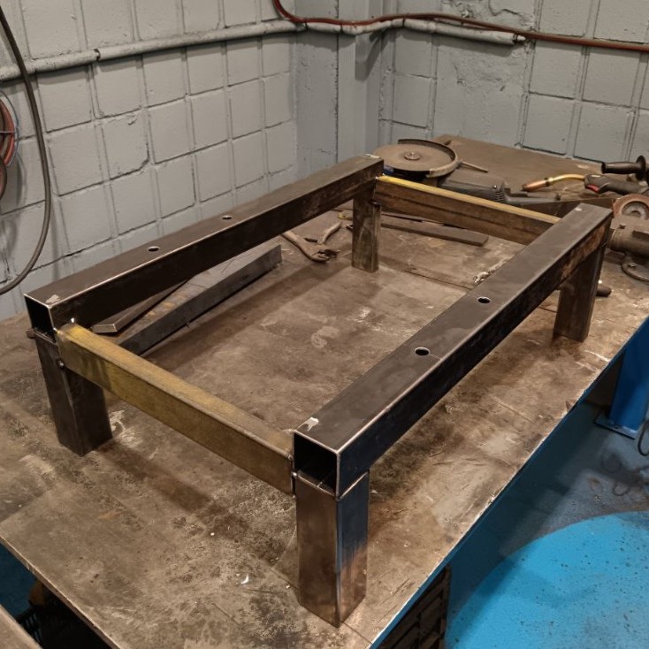
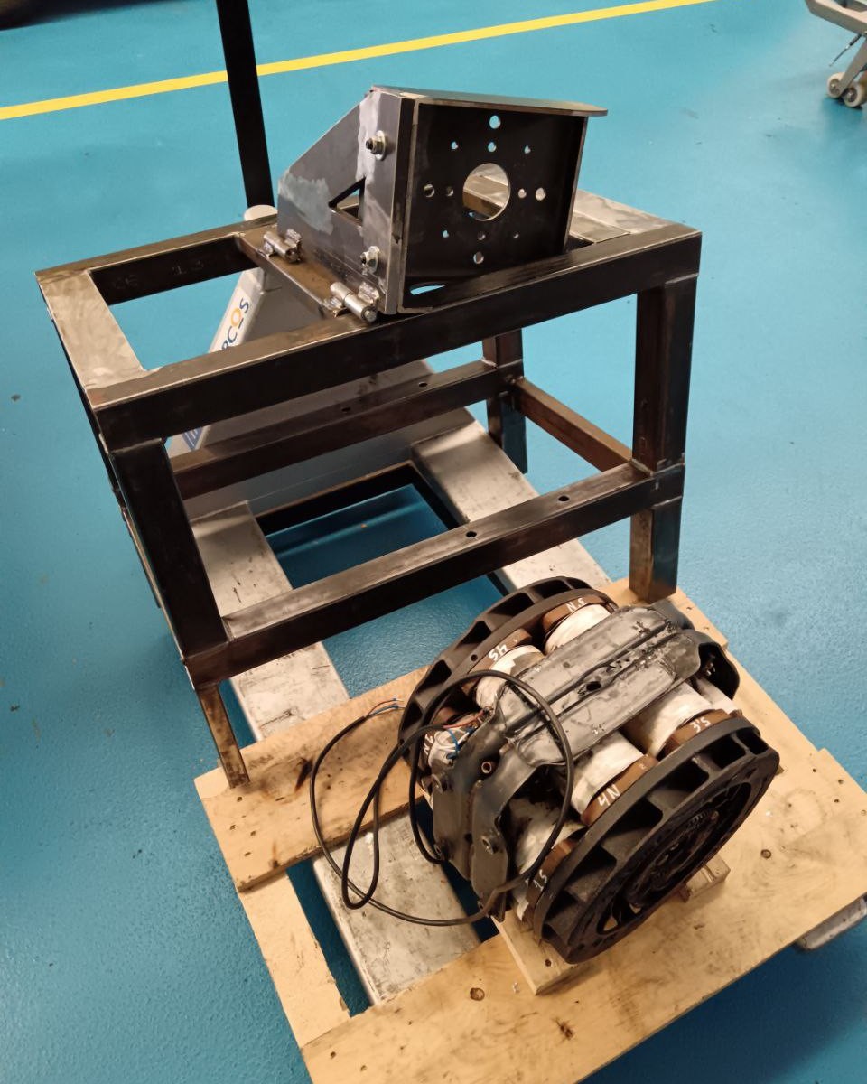
I wanted to use materials I already had available in my workshop. This is the main reason why the frame uses different steel profiles like 40x40mm and 40x20mm pipes. I also reused a motor holder that we manufactured a few years ago for a previous electric motorcycle project. Since I had disassembled the eddy current brake for cleaning and restoration, it was much easier to take precise measurements and draw all the parts in CAD.
The first thing I designed was the structure. I used the old pipes to draw a base to support the brake. Above that base I added another structure where the electric motors would be mounted.
A load cell is a transducer that converts mechanical force into an electrical signal. In a dynamometer it measures the reaction force of the brake. This data allows the software to calculate the torque produced by the motor. Most load cells use strain gauges arranged in a Wheatstone bridge circuit to detect very small deformations in the metal body of the sensor.
One of the most important factors in the design is the placement of the load cell. It must be perfectly aligned with the axis of the brake so the applied torque creates a force at an exact 90 degree angle. Furthermore the distance from the center of the eddy current brake changes the requirements. If the load cell is placed further away from the center of rotation it will measure less force at that position. This means a load cell with a smaller capacity can be used which helps maintain precision. If the load cell is placed very close to the brake a larger capacity model is required to measure the same amount of torque.
The following examples show how the required capacity changes for a torque of 100 Nm applied to the brake:
\[T = F \cdot r\]Where:
- $T$ is the Torque ($100 \text{ Nm}$)
- $F$ is the force applied to the load cell in Newtons
- $r$ is the lever arm length in meters
Load cell at 100 mm
At this position the lever arm is very short so the force needed to counteract the torque is high.
\[F = \frac{100 \text{ Nm}}{0.1 \text{ m}} = 1000 \text{ N}\]With this force the load cell would need to support a minimum mass of:
\[m = \frac{1000 \text{ N}}{9.81 \text{ m/s}^2} = 101.94 \text{ kg}\]Load cell at 500 mm
As the distance from the center of rotation increases the force decreases proportionally. In this configuration the force is reduced by a factor of five compared to the 100 mm setup which makes the system much easier to manage mechanically.
\[F = \frac{100 \text{ Nm}}{0.5 \text{ m}} = 200 \text{ N}\]With this force the load cell would need to support at least the following mass:
\[m = \frac{200 \text{ N}}{9.81 \text{ m/s}^2} = 20.39 \text{ kg}\]Load cell at 1000 mm
At a distance of one meter the magnitude of the force in Newtons numerically matches the value of the torque in Nm.
\[F = \frac{100 \text{ Nm}}{1.0 \text{ m}} = 100 \text{ N}\]With this force the load cell would need to support a minimum mass of:
\[m = \frac{100 \text{ N}}{9.81 \text{ m/s}^2} = 10.19 \text{ kg}\]It is important to keep in mind that load cells generally become more expensive as their weight capacity increases. In my case I decided to place the load cell at 500 mm from the center of the eddy current brake. This was a balance between the physical dimensions of the frame and the overall cost because I did not want to build an oversized structure. If we assume the maximum rated values for the eddy current brake which is 1000 Nm we can calculate the necessary load cell capacity:
\[F = \frac{T}{r}\] \[F = \frac{1000 \text{ Nm}}{0.5 \text{ m}}\] \[F = 2000 \text{ N}\]Calculating this in kg:
\[m = \frac{F}{g}\] \[m = \frac{2000 \text{ N}}{9.81 \text{ m/s}^2}\] \[m = 203.87 \text{ kg}\]With this configuration I would need a load cell that supports a minimum of 200 kg to handle the full 1000 Nm. I am not going to reach that level of torque with my current electric motor because as we will see later, the torque is reduced by the gear ratio of the chain drive.
Let’s calculate the specific case for the motor I am using which has the highest torque in my collection. According to the datasheet it has a peak torque of 140 Nm and can reach speeds up to 6000 RPM. For this reason the first thing I need to calculate is the ratio between the motor sprocket and the brake crown so that the eddy current brake does not exceed its 4500 RPM limit when the electric motor is spinning at 6000 RPM.
The formula for the speed relationship is:
\[N_{motor} \cdot Z_{pinion} = N_{brake} \cdot Z_{crown}\]Where:
- $N_{motor}$ is the maximum motor speed (6000 RPM)
- $Z_{pinion}$ is the number of teeth on the motor sprocket (unknown)
- $N_{brake}$ is the maximum allowed speed of the brake (4500 RPM)
- $Z_{crown}$ is the number of teeth on the brake crown (24)
Using the formula to solve for the motor sprocket:
\[Z_{pinion} = \frac{N_{brake} \cdot Z_{crown}}{N_{motor}}\]I am using a crown with 24 teeth because it is one of the smallest sizes that fits on the 50 mm diameter shaft that I am manufacturing:
\[Z_{pinion} = \frac{4500 \text{ RPM} \cdot 24}{6000 \text{ RPM}}\] \[Z_{pinion} = \frac{108000}{6000}\] \[Z_{pinion} = 18\]To give the system a bit of a safety margin I decided to use a sprocket with 17 teeth instead of 18.
With this relationship established I can calculate the maximum torque that the eddy current brake and the load cell will experience when using this specific motor.
\[i = \frac{Z_{crown}}{Z_{pinion}} = \frac{24}{17} = 1.411...\] \[T_{brake} = T_{motor} \cdot i\]Torque in the brake:
\[T_{brake} = 140 \text{ Nm} \cdot 1.411 = 197.54 \text{ Nm}\]Torque applied to the load cell:
\[T_{load\_cell} = T_{brake} = 197.54 \text{ Nm}\] \[F = \frac{T_{brake}}{r} = \frac{197.54 \text{ Nm}}{0.5 \text{ m}} = 395.08 \text{ N}\]Mass applied to the load cell:
\[m = \frac{F}{g} = \frac{395.08 \text{ N}}{9.81 \text{ m/s}^2} = 40.27 \text{ kg}\]This means that I could use a smaller load cell than 200 kg but since the mechanical system can support up to 500 hp (excluding the chain) I wanted to design the whole system dimensioned for that power.
With this information I was finally ready to design the complete system:
 Structure
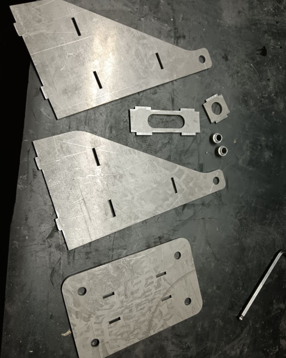
The reaction arm that transmits the torque between the eddy current brake and the load cell was manufactured using 5mm thick laser cut sheet metal which was later assembled and welded as shown further down.
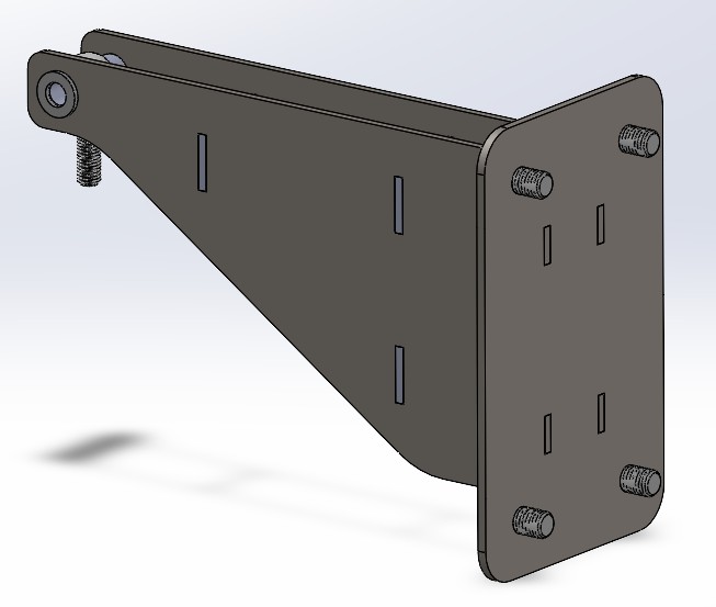 Load Cell Arm
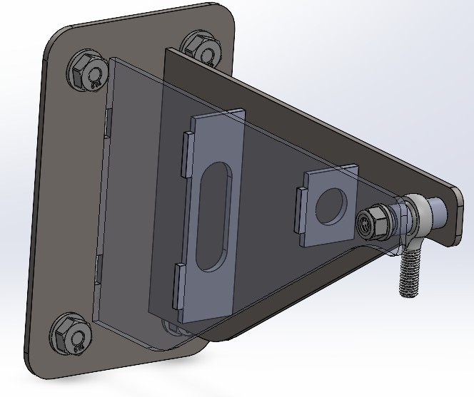 Load Cell Arm
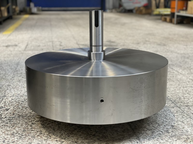
The next critical step was to design the shafts that would support the weight of the eddy current brake.
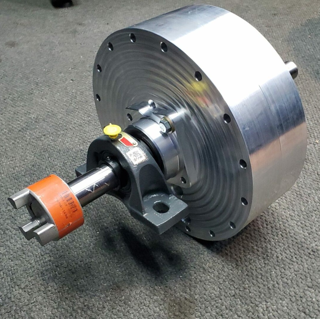
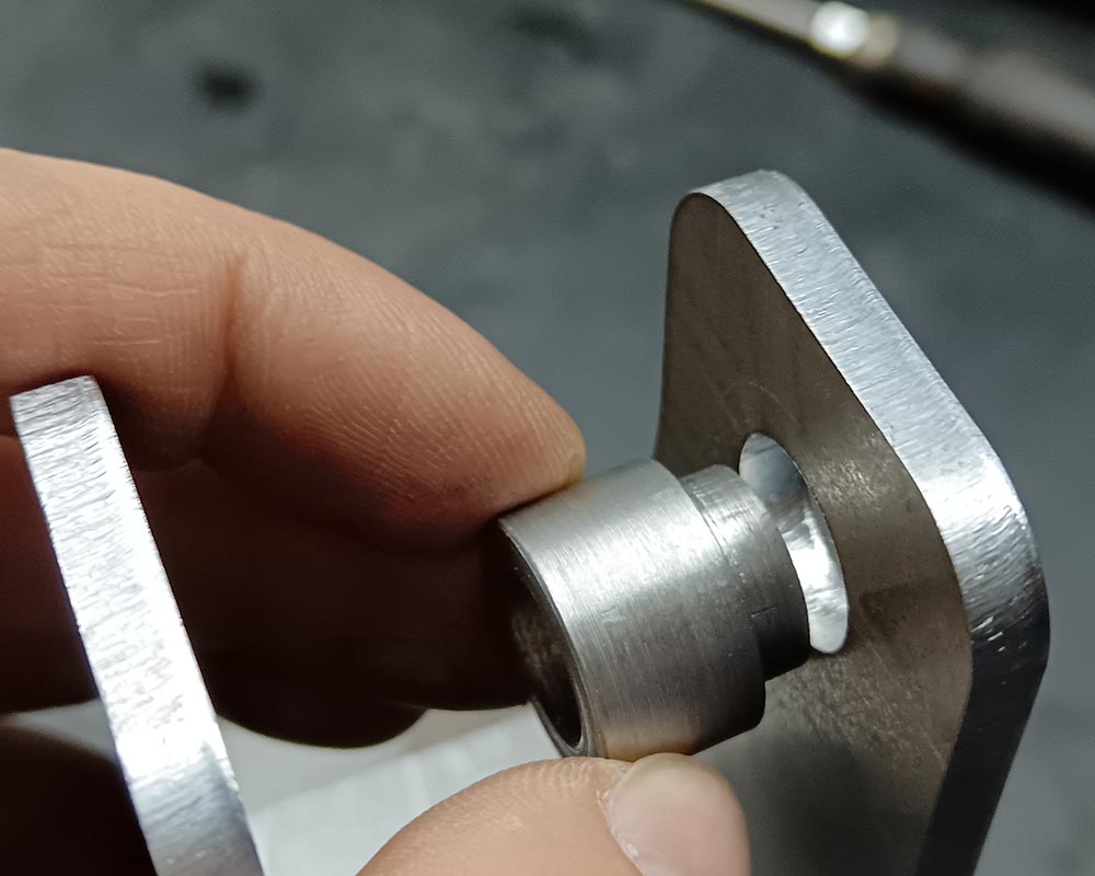
Shaft Coupling
As shown in the image, this is the original coupling. In a truck these brakes are normally mounted with a universal joint or cardan shaft on each side. They use a specific self-centering coupling with a serrated or “fluted” pattern to ensure perfect alignment under heavy loads.
In my case using the original parts was not an option since I did not have them and manufacturing that specific serrated pattern would be extremely expensive.
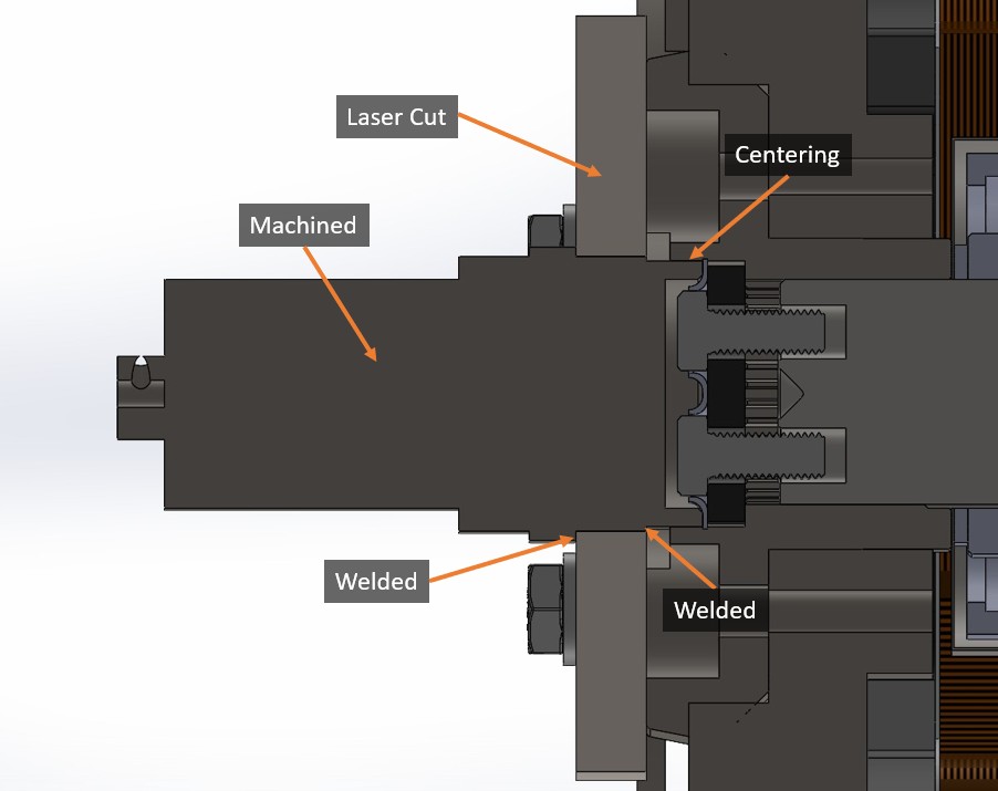
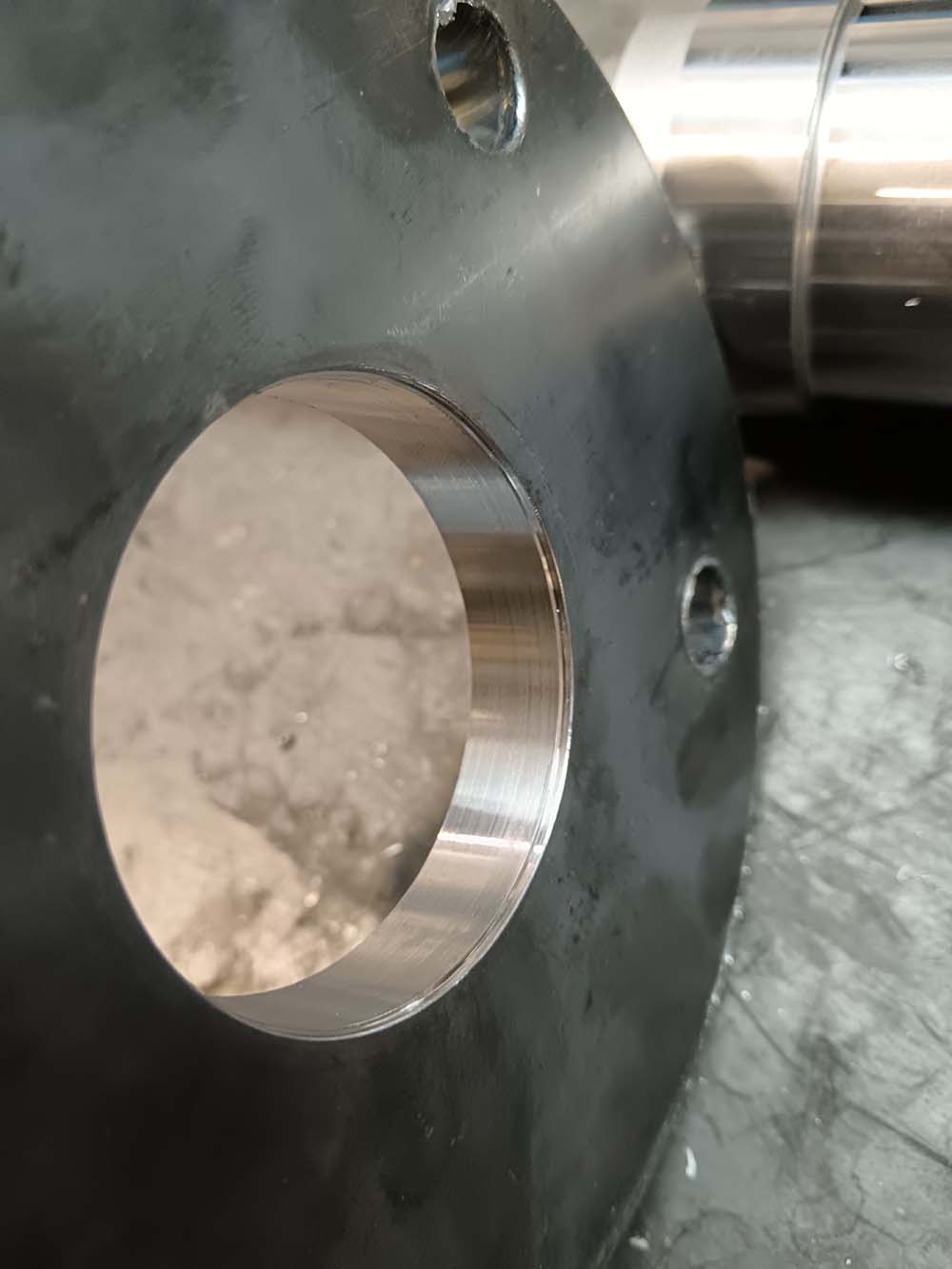
After disassembling and cleaning the unit I looked for an alternative solution. I noticed that the face marked in the image was factory-machined at the same time as the rear faces where the rotors are mounted. This meant it was a valid reference point for centering the new custom shafts. This face would serve as the guide to center the external couplings that allow the eddy current brake to rest on the main bearings.
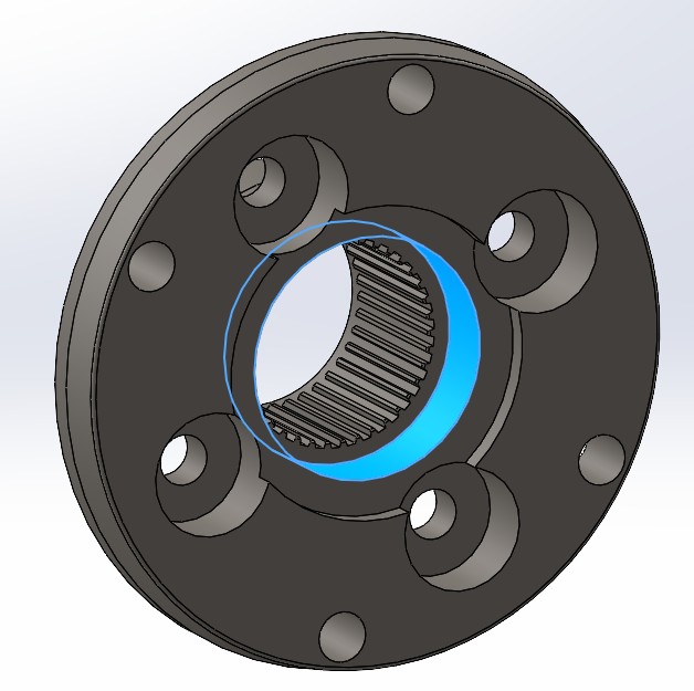 Centering Face
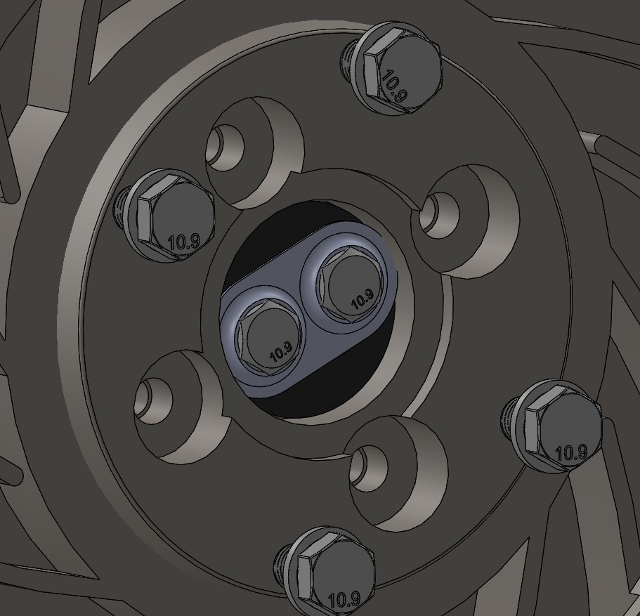
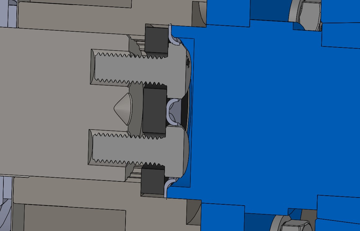
One detail to consider was the limited space available for centering. As seen below there is a light gray metal plate acting as a locking tab. Its purpose is to prevent the screws that adjust the internal bearings from loosening since they are not fully tightened to allow for thermal expansion. After careful measurements I confirmed there was just enough margin to use that inner face as a centering pilot for the new shaft.
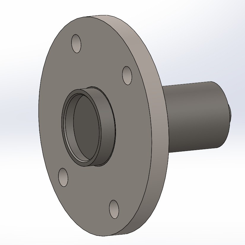
 Shaft Coupling in CAD
 Shaft Coupling in CAD
 Shaft End in CAD
The next decision was to figure out how to manufacture these parts.
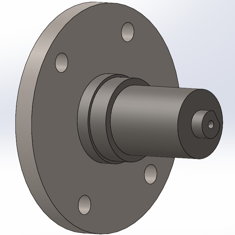 End Shaft Design
 End Shaft Design
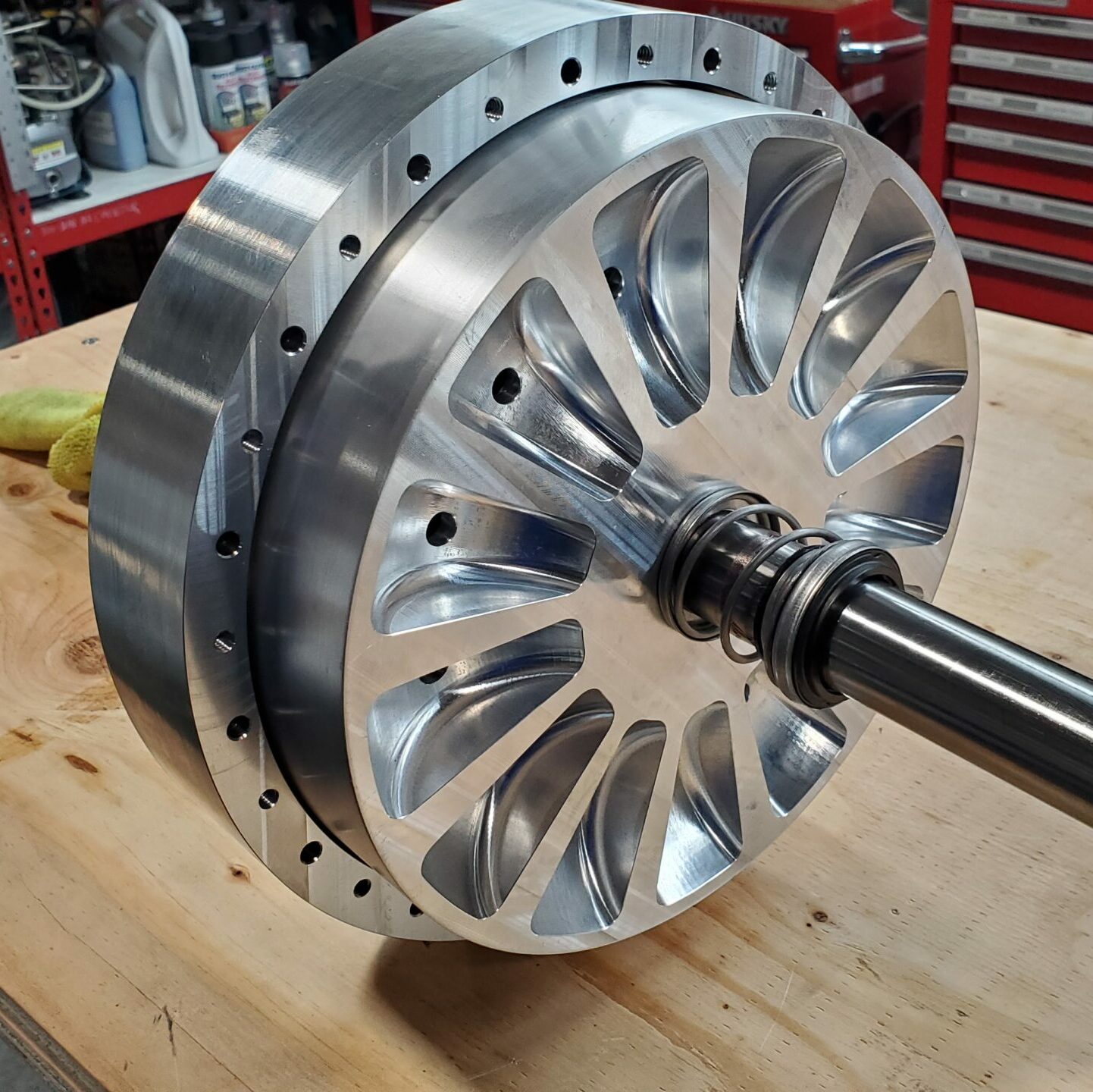
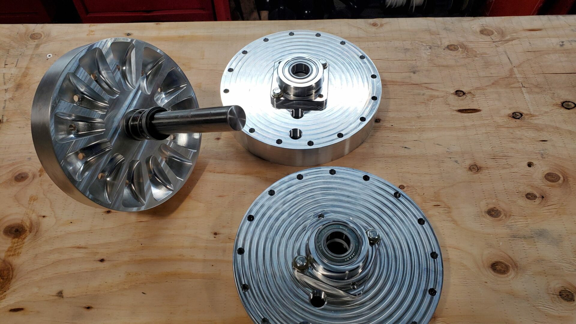
I had access to a manual lathe but removing all that material from a solid block would have been a massive amount of work and time. The largest outside diameter was 165 mm and the bearing support was 50 mm. To solve this I decided to split the parts into two pieces: a turned shaft and a 15 mm thick laser-cut steel disc. Once both were ready I would press-fit one into the other and then weld them together as shown in the cross-section below:
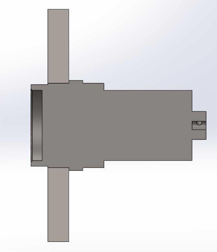 End Shaft CAD Design
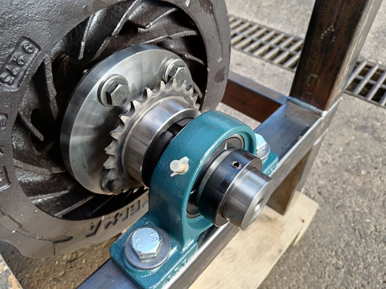
With this design finished I could proceed with the next step which was the chain coupling. To transmit the power from the motor to the eddy current brake I decided to use a conical taper lock coupling.
 Chain Coupling System
These couplings consist of two tapered pieces as shown in the image. The hole indicated by the green arrow has a thread on the outer part and a seat on the inner part. When the screw is tightened the inner black piece moves to the left while the outer gray piece moves to the right. The black piece has a slit that allows it to compress and grip the shaft diameter perfectly. This way the piece adapts and tightens itself onto the shaft.
With this type of coupling I did not need to perform any special machining on the shaft. It includes a keyway if necessary but for the relatively low power I am transmitting with the electric motor it was not required.
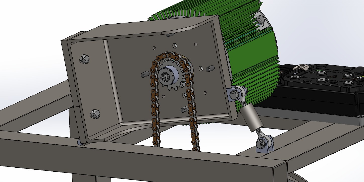
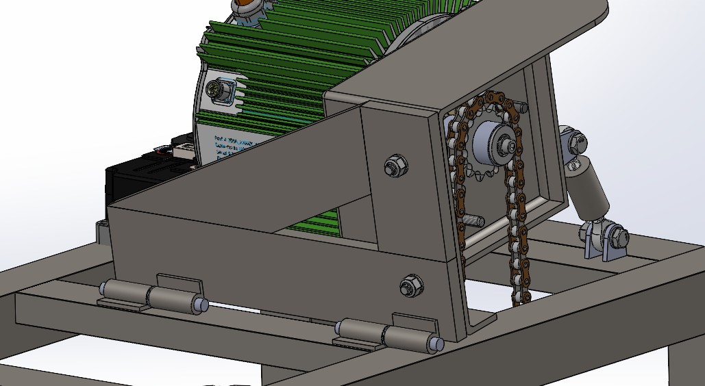
 Complete Structure
 Complete Structure
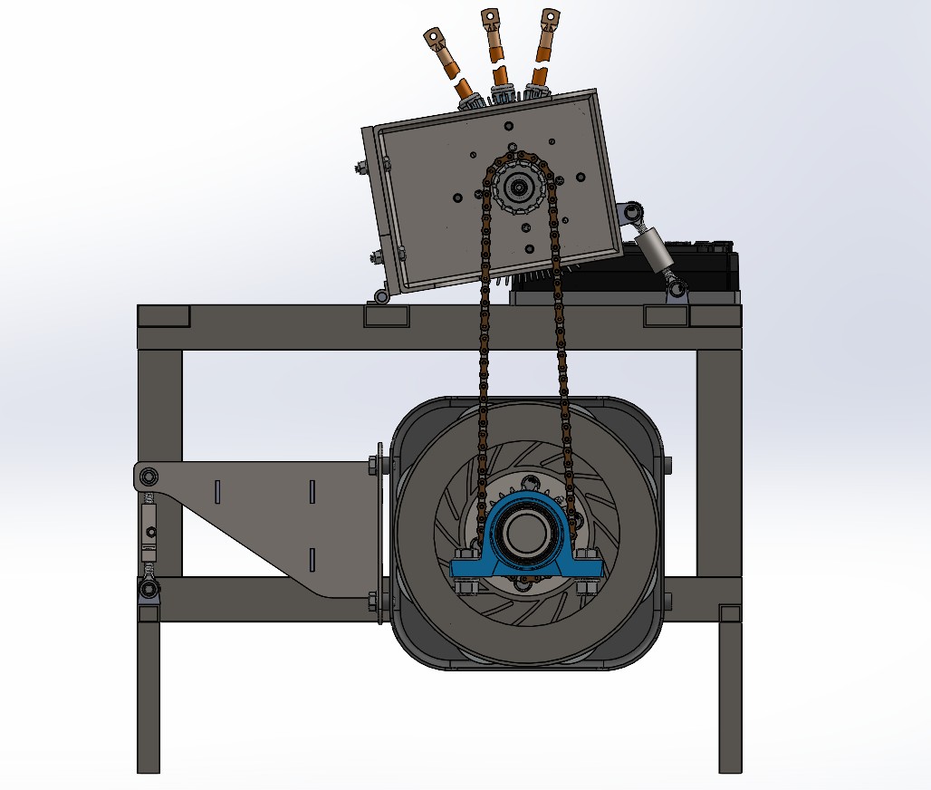
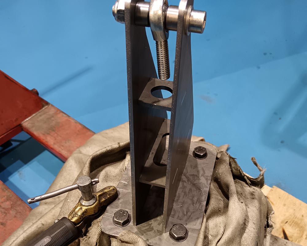
Finally the last part was the design of the motor tensioner. My plan was to test two different motors: one with a maximum speed of 6000 RPM and another capable of reaching 8000 RPM. This meant I would need to mount two different sprockets so the chain tension must be adjustable to accommodate those changes.
The motor support plate was a reused component so I had to adapt it to the new frame design. It basically sits on two hinges that allow it to pivot. The tensioning system consists of two rod ends with opposite threads which create a turnbuckle effect. By rotating the center link I can pull the motor into position and then tighten the jam nuts to prevent anything from loosening due to vibrations.
 Motor Holder
 Motor Holder
Manufacturing
With the design ready and all the CAD drawings finished I started to manufacture it.
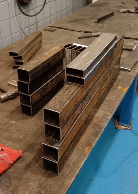 Cut Structure
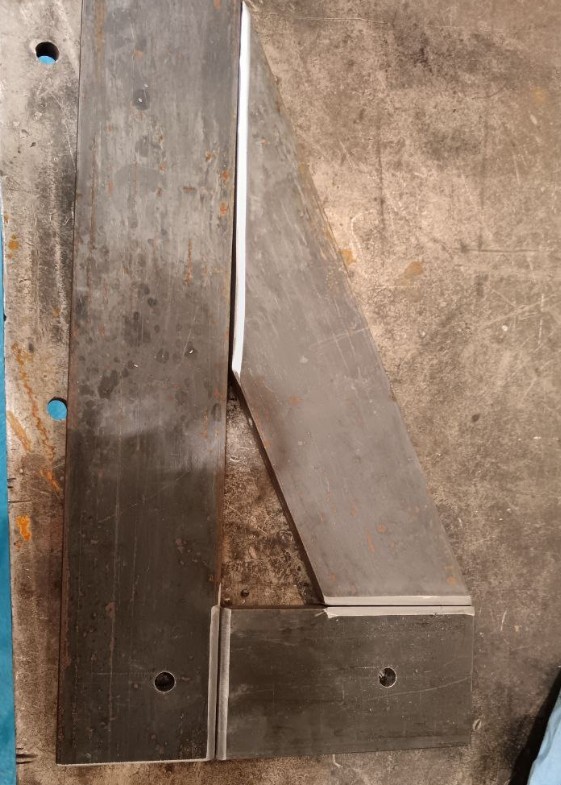 Motor Holder ready to weld
 Welding Structure
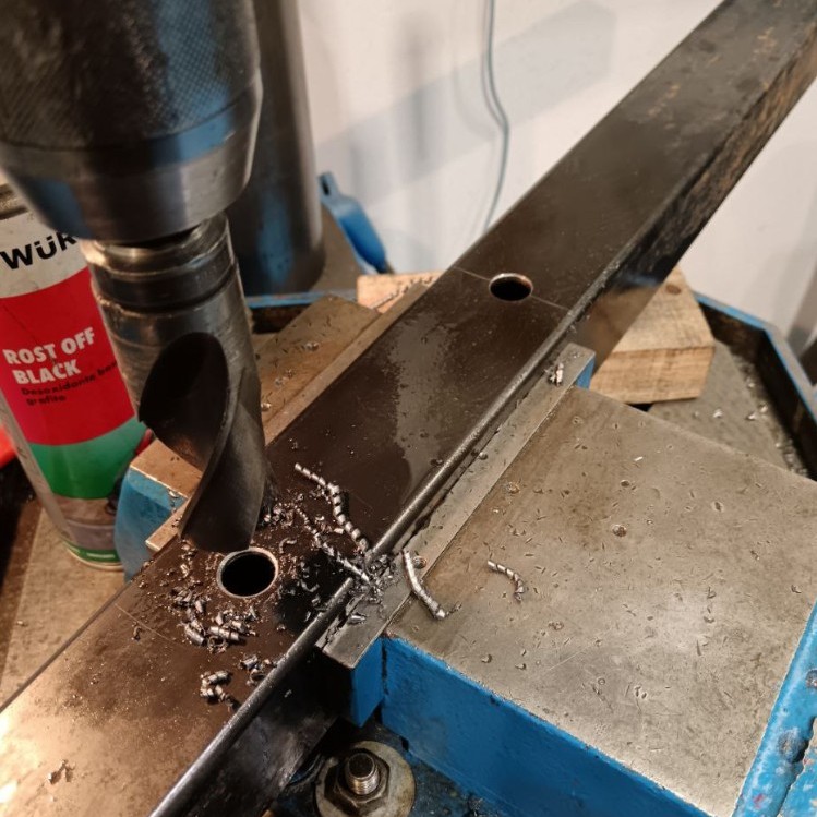 Holes for bearings
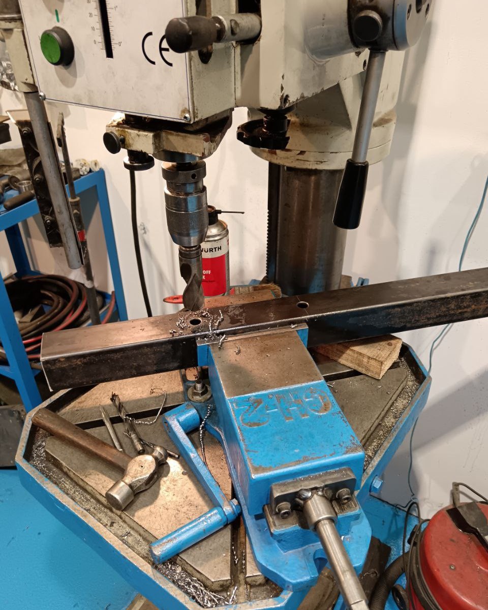 Drilling holes for bearings
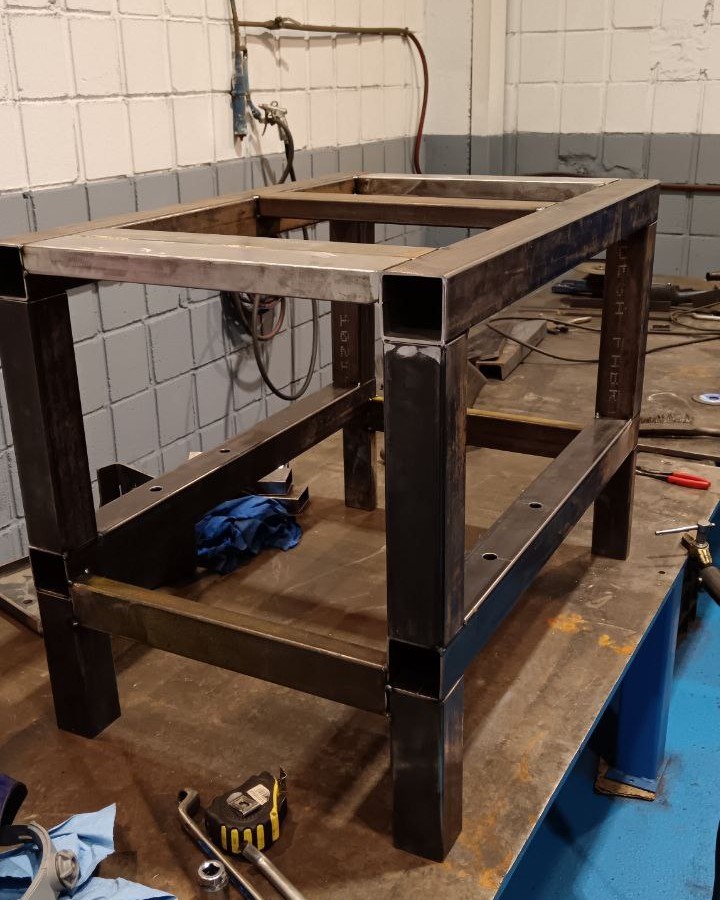 Structure ready to weld
The arm to transmit the torque to the load cell was manufactured with laser cutting. I adjusted the holes to make it fit perfectly before welding it.
 Laser cut arm for load cell
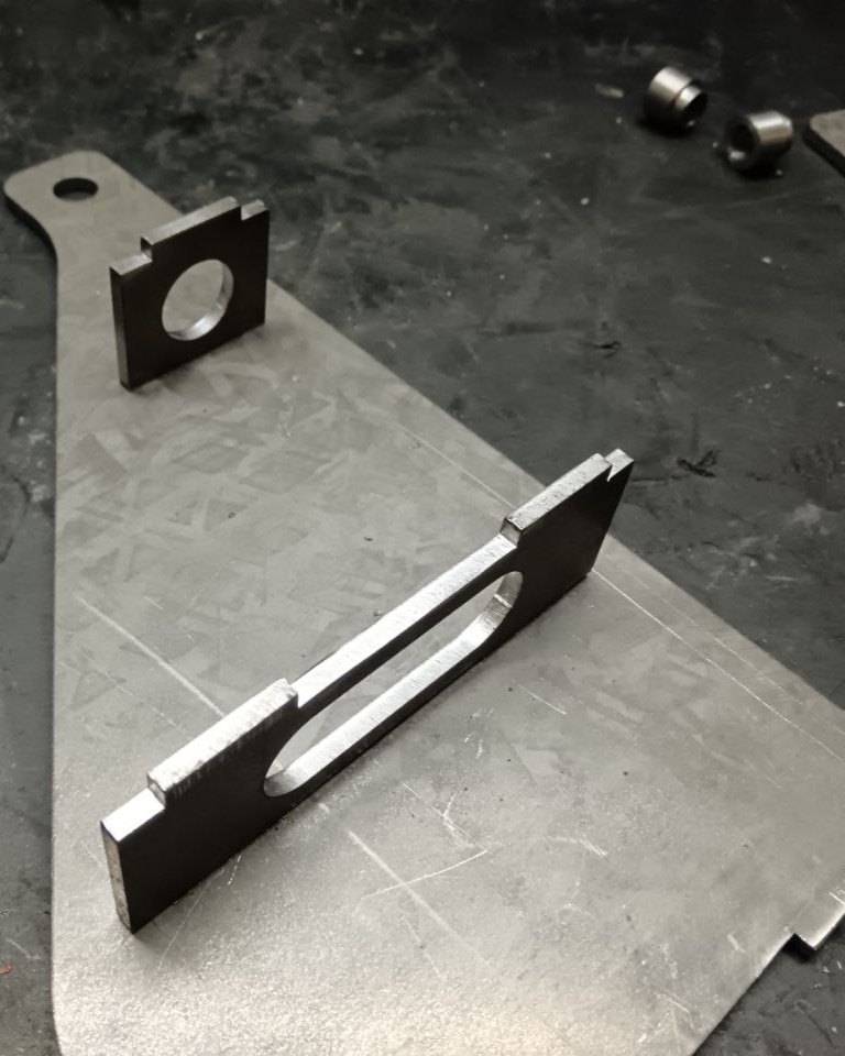 Laser cut arm for load cell
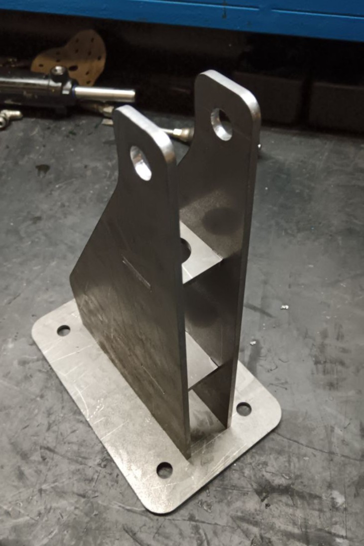 Assembled arm
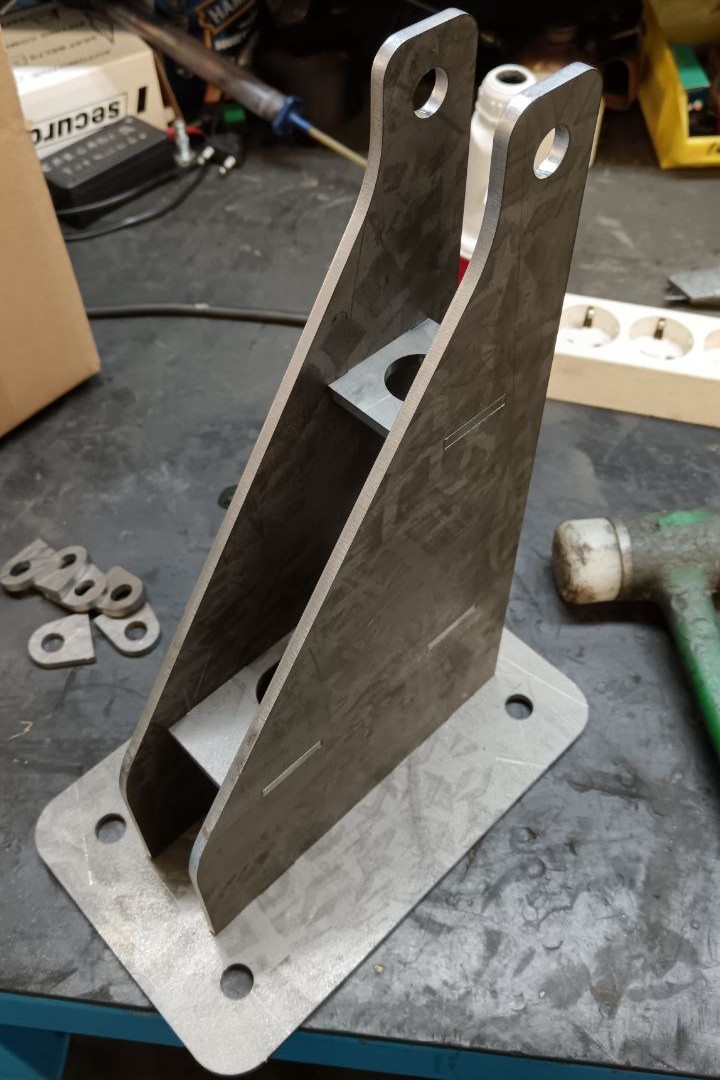 Assembled arm
 Bushing for load cell
 Welding the arm
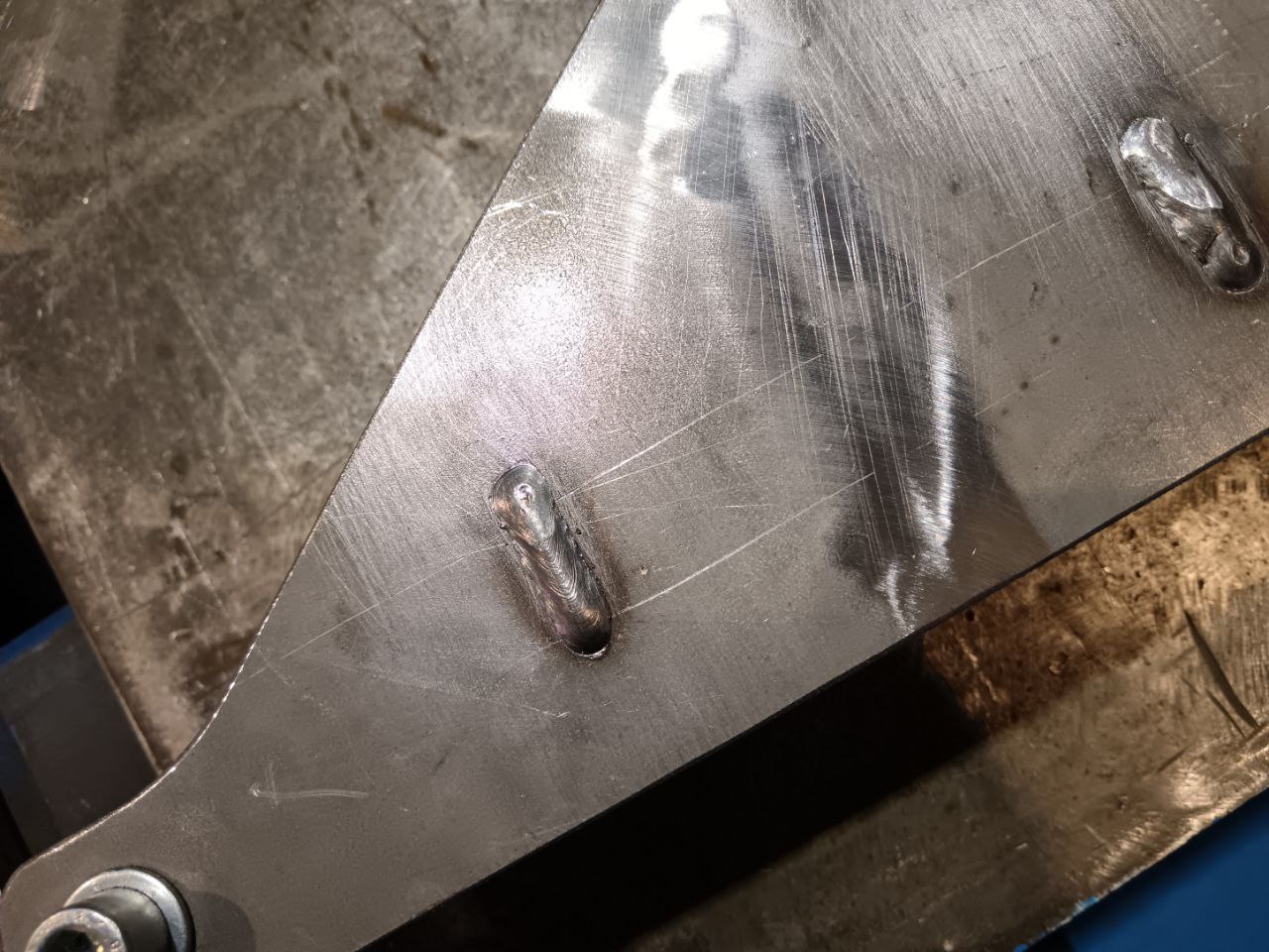 Welded arm
 Raw shaft
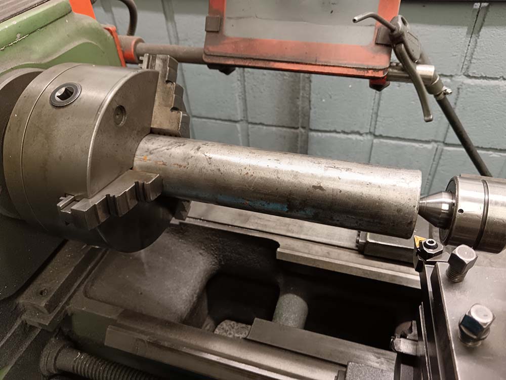
To manufacture the shaft ends that will hold the brake weight, as explained previously it has been manufactured from two different pieces. A raw steel bar and a laser cut disc. First, I machined the bar but leaving some material in all faces.
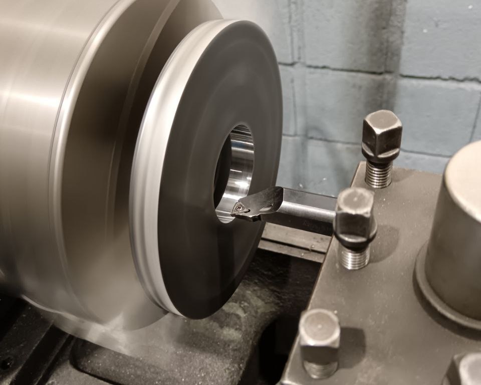 Grinding internal diameter of laser cut
 Raw shaft
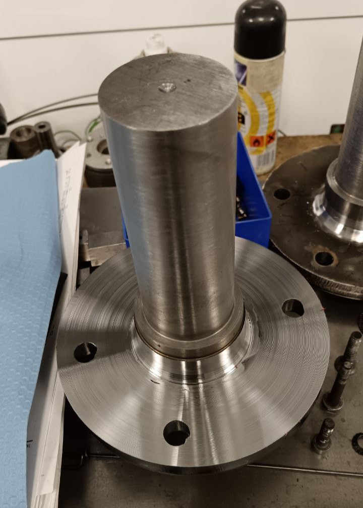
To assemble both parts I left a bit interference between the shaft and the disc so I heated the disc and froze the shaft. After assembling it, when both pieces returned to the normal temperature they were perfectly fitted.
 Shaft Manufacturing
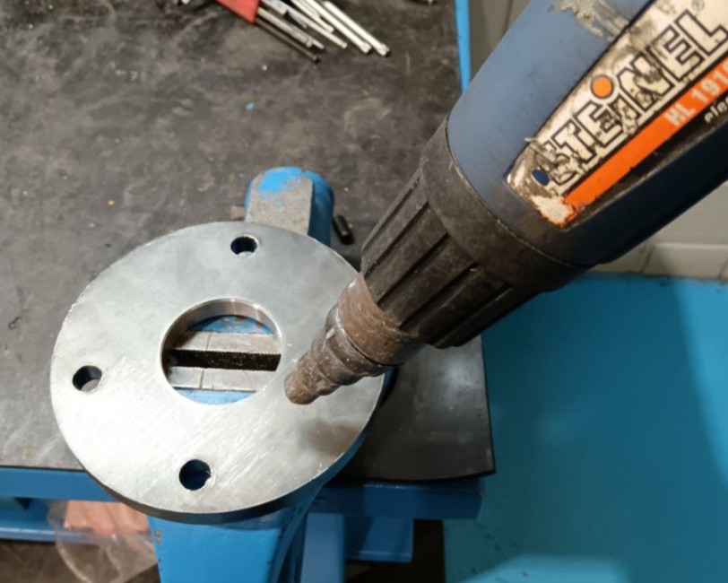 Heating disc for interference assembly
 Internal hole of the laser-cut after lathe
 Shaft ready to mount
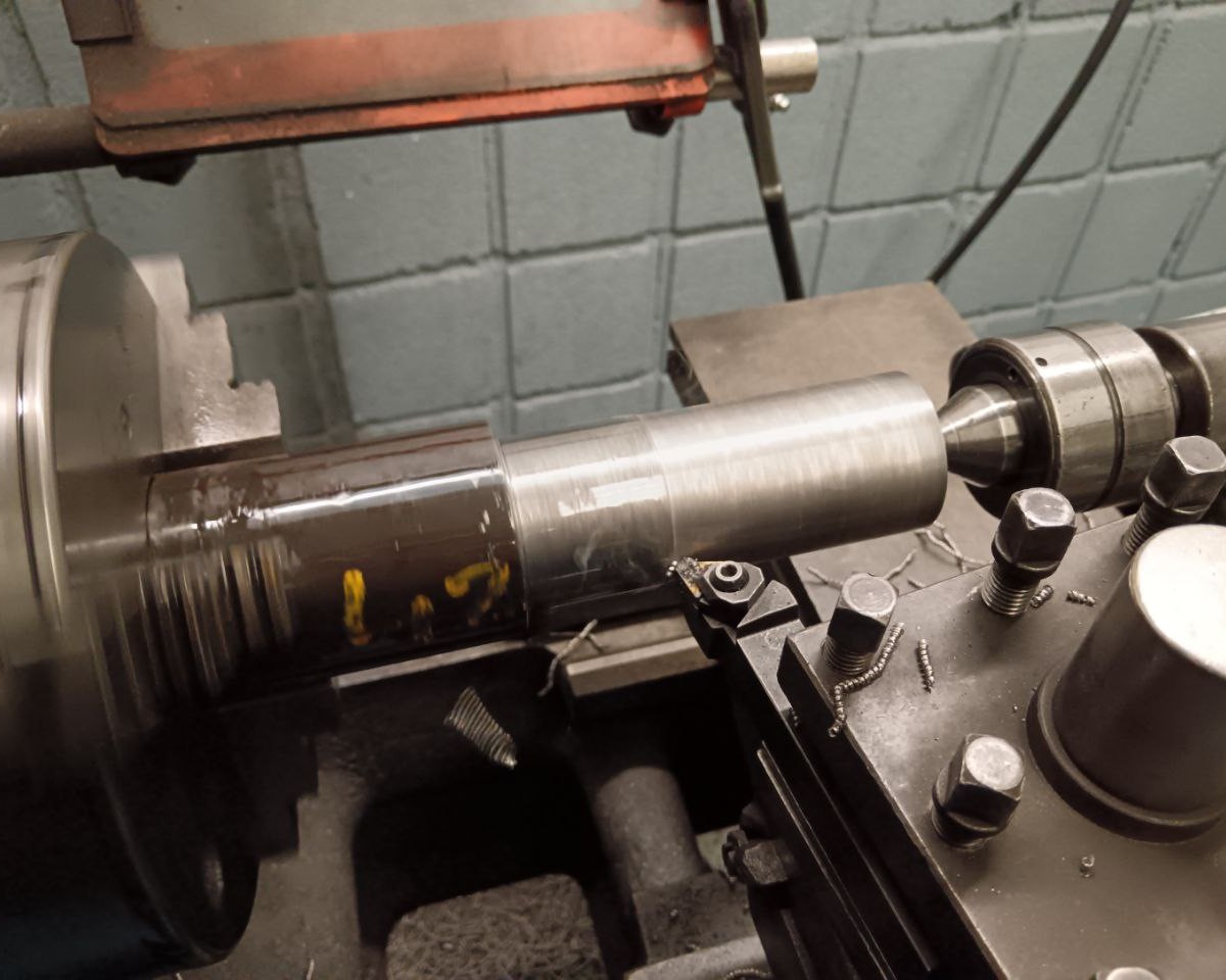
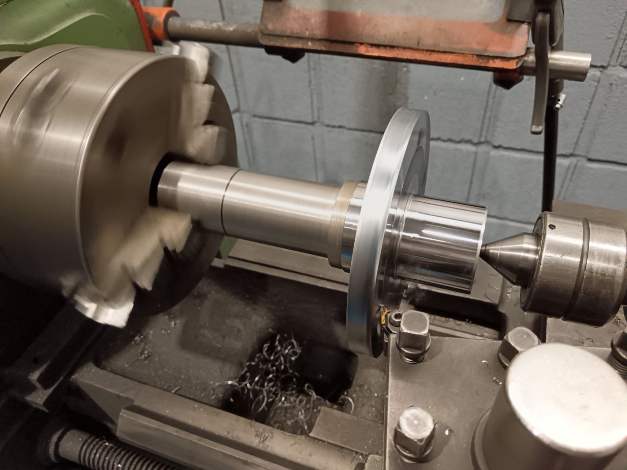
Now it was important to machine all the faces again after welding as the welding can deform some parts. I left enough material to do it.
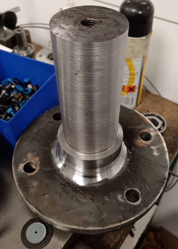 Shaft Manufacturing
 Shaft Manufacturing
After that I checked that all the faces were correctly aligned between them with a comparator.
 Shaft Manufacturing
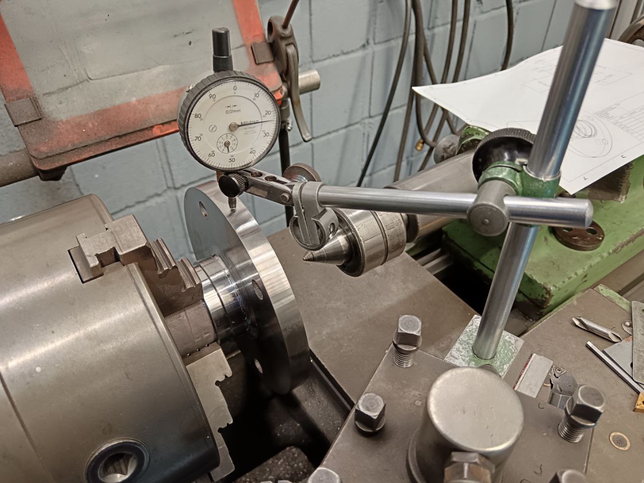 Checking the centering
 Welded Structure
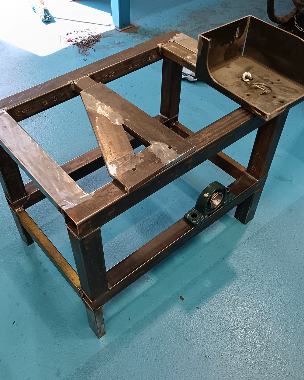 Welded Structure
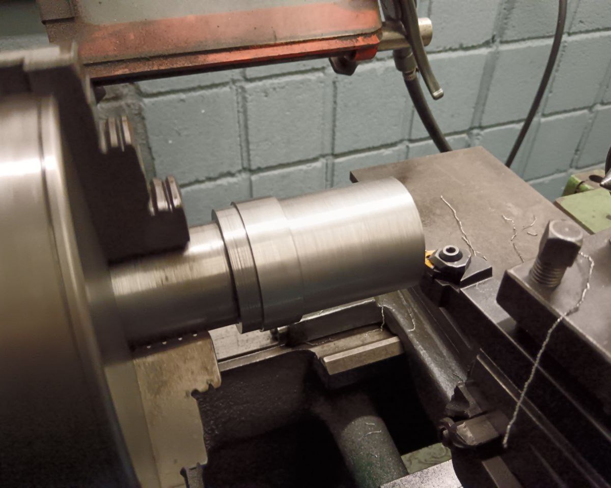
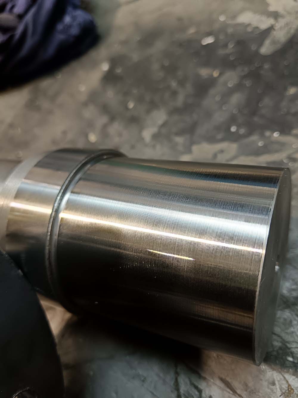
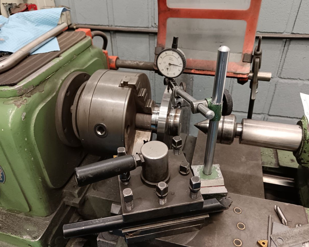 Finishing shaft ends in the lathe
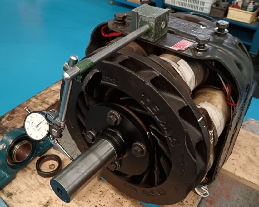 Checking the centering of the axis
After that, I proceeded to assemble everything:
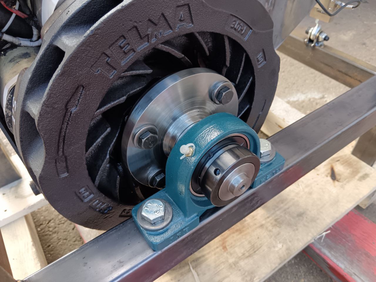 Encoder Side Bearing
 Chain Side Bearing
 Assembled Brake
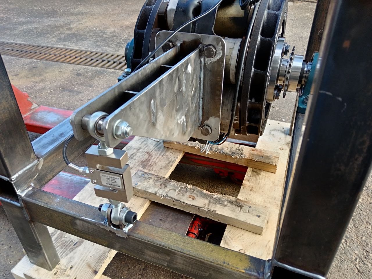 Load Cell Arm
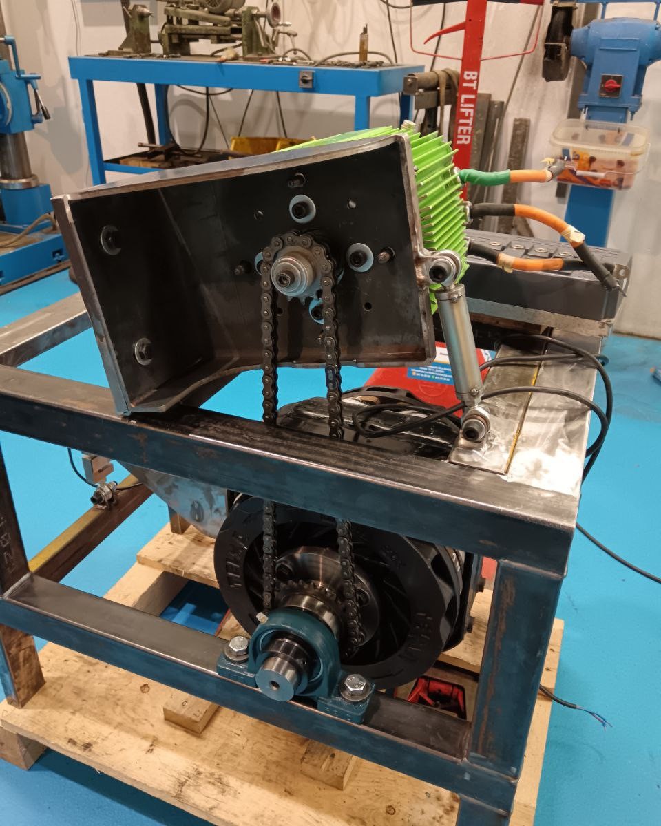 Chain Tensioner Installed
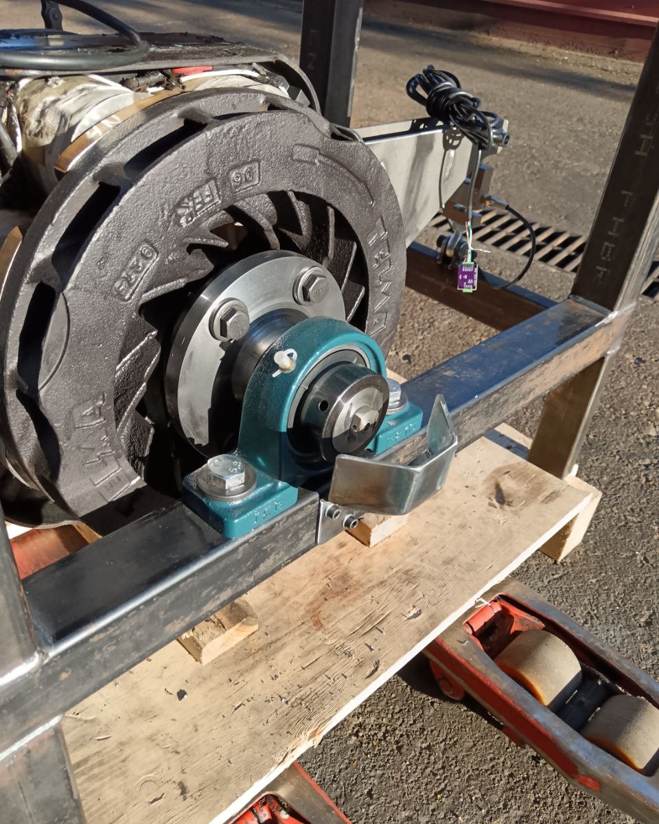 Encoder Protector Installed
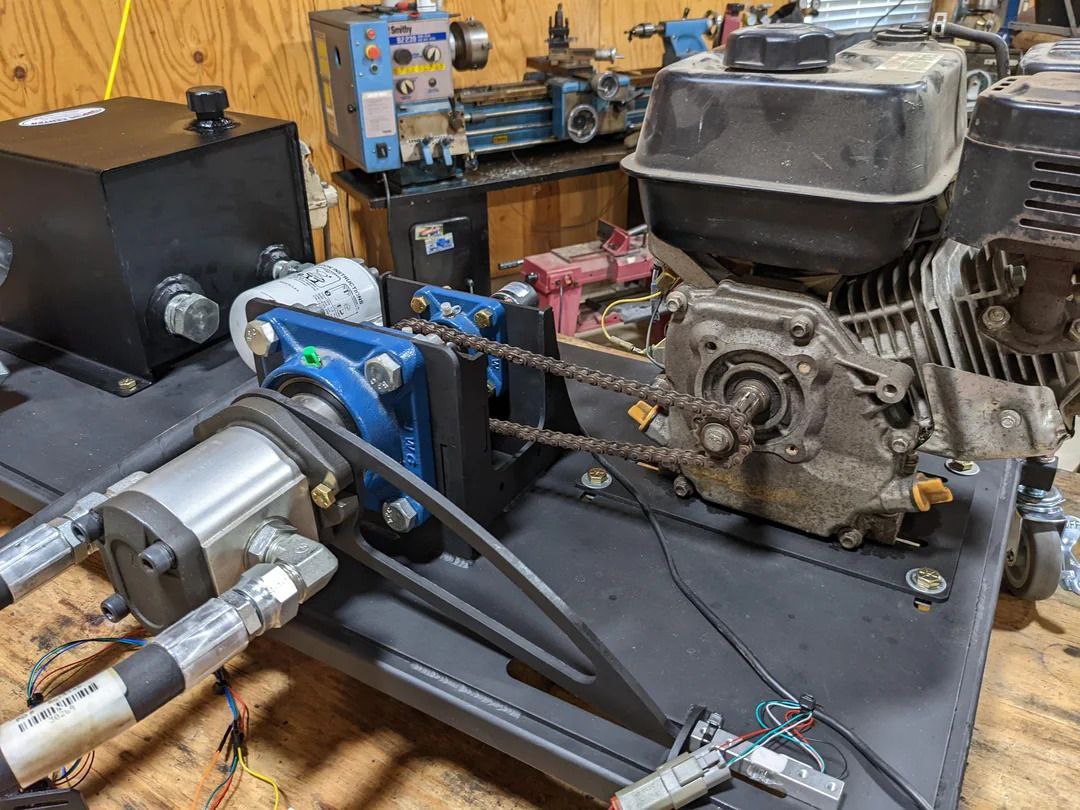
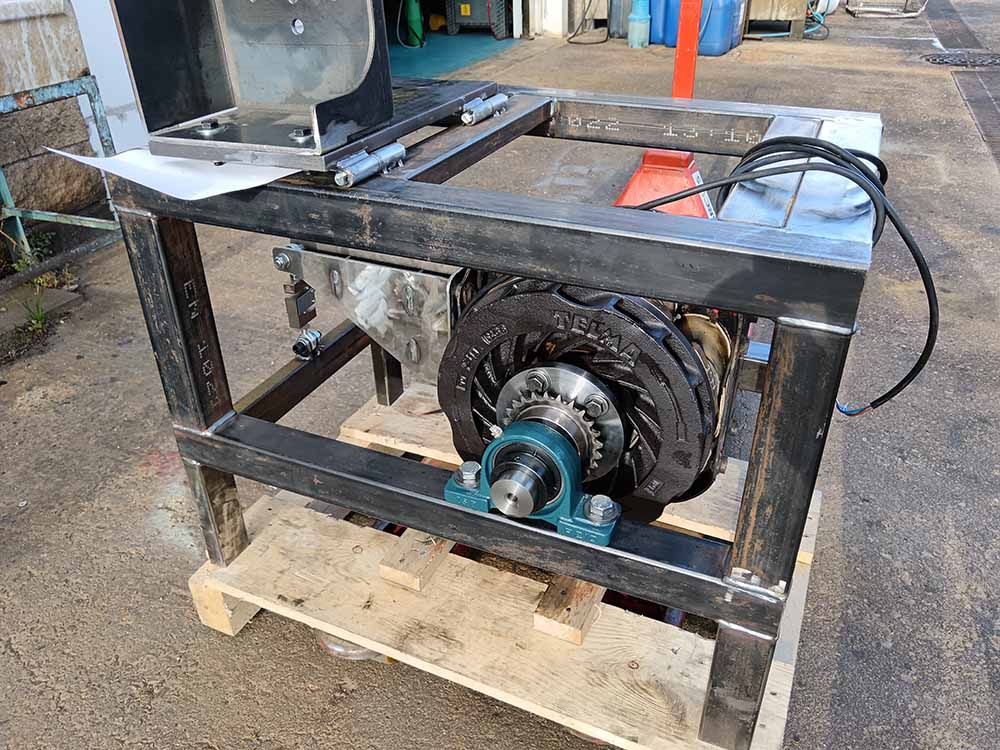
With everything assembled the dyno was ready to spin.
One problem that took me a surprisingly long time to diagnose was chain vibration. The chain I was using was not new and it was stretched. It wasn’t meshing properly with the sprockets, which were causing noise, vibrations, and heat. I wasted time diagnosing noise in the sensors and trying to filter it, but that wasn’t the root cause. The root cause was a faulty mechanical component.
What I mean by this is that it’s always important to make sure you fix problems at the earliest stage, following the order: Mechanics > Hardware > Software. It’s important to have properly functioning mechanics, if you have a problem, it’s often easier to fix it than trying to apply filters or patches at later stages. After changing the chain with a new one, all my vibrations were solved.
Imagine how problematic it was that, while tuning the electric motor’s inverter, the current PI control was also noisy, leading me to believe it was incorrectly configured. After replacing the chain, all those problems were resolved.
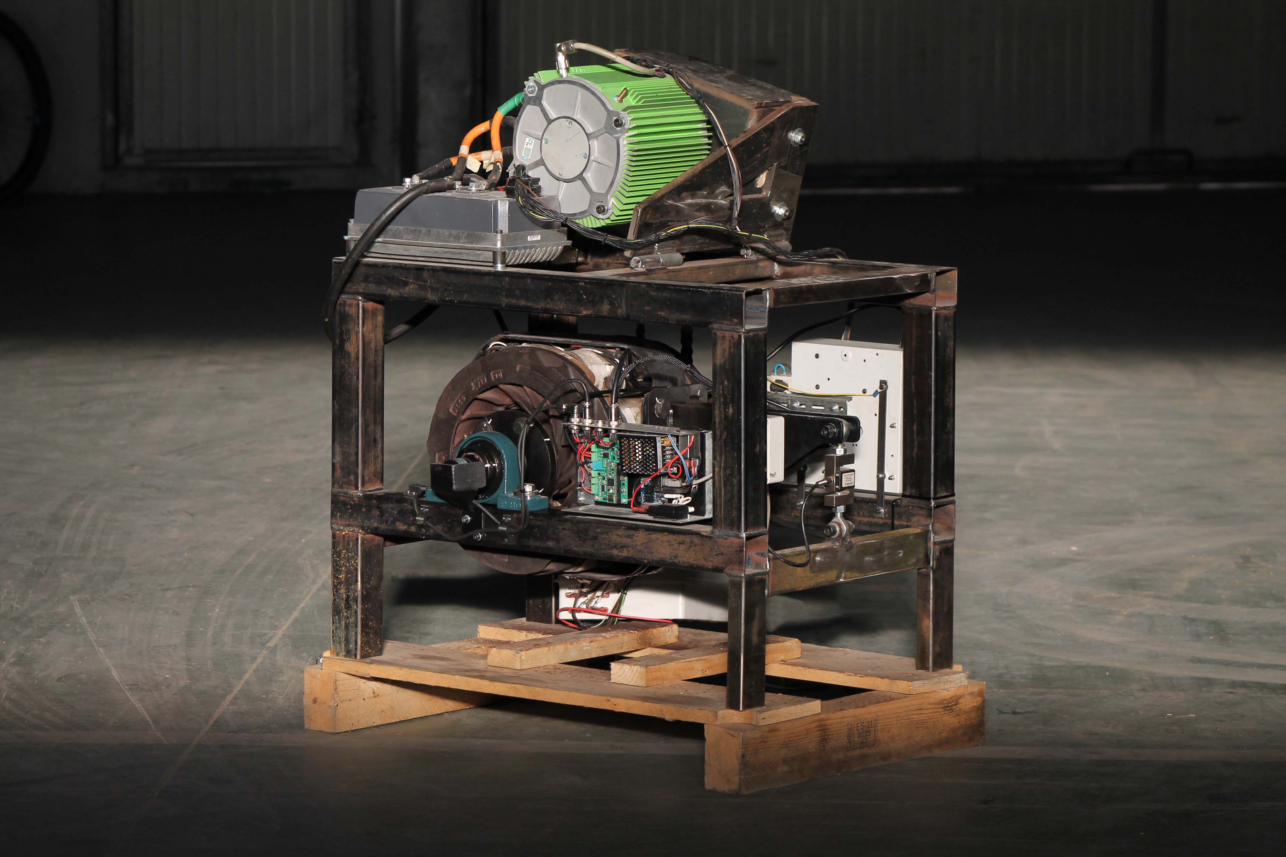
Final Result
Electronics ⚡
With all the mechanical part ready it was time to start with the electronics and software. This was going to be the hardest part of the project. When I started it I thought that in two months I could have it finished. Unfortunately, that wasn’t what happened.
System Architecture
Before starting the build I needed to establish a clear system architecture. To keep the project manageable and robust I decided to split the design into three different layers.
The Power Stage
Starting at the lowest level I needed a system to control the electrical energy being sent to the eddy current brake. The coils in the retarder require a significant amount of current to generate a strong enough magnetic field for braking. This stage is responsible for high-current switching and power regulation.
The Logic and Control Stage
The next layer is the “brain” of the dynamometer. This stage handles all the logical calculations and sensor data acquisition. It reads the signals from the encoder for speed, the load cell for torque, and various temperature sensors to monitor the status of the system.
Crucially this stage must operate in real-time. It executes the PID (Proportional-Integral-Derivative) control loop at a relatively high frequency to ensure the brake responds instantly to changes in torque or motor speed. I will explain the inner workings of the PID controller in a later section.
I considered integrating the power and logic stages onto a single PCB but I decided not to do it for two main reasons:
- Flexibility: Separating them means that a design error or a modification in one section does not require me to redesign and manufacture the entire assembly.
- Signal Integrity: As we will see later these power stages emit a significant amount of Electromagnetic Interference (EMI). Physically separating the logic from the high-power switching helps prevent electrical noise from corrupting the sensitive sensor data.
The User Interface
Finally I needed a way for the user to interact with the machine. For the software side I chose a client-server web architecture. By hosting a small web server directly on the control unit any device with a browser can act as the dashboard. This eliminates the need to install specific software or drivers on a laptop and allows for a clean wireless connection via Wi-Fi.
With this structural roadmap defined I was ready to start developing each component in detail.
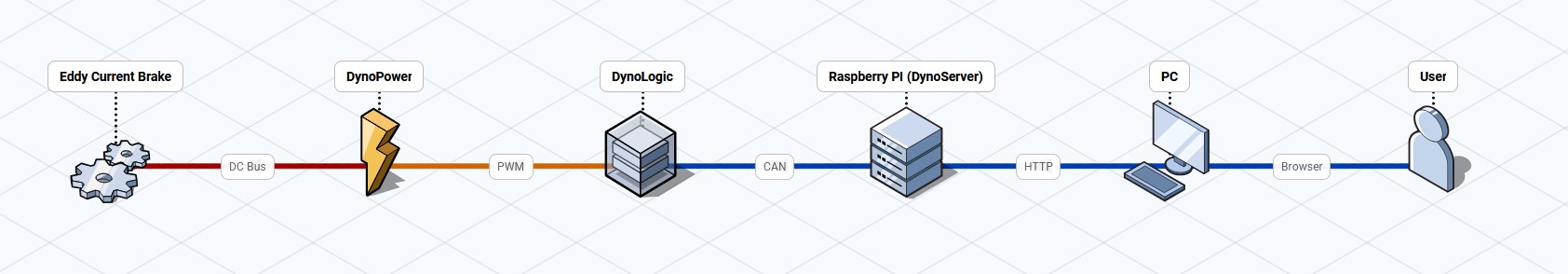 System Architecture
First, let’s analyze the electrical specifications of the eddy current brake that I was going to use.
Telma AC 51 - 00
Electrical Characteristics of Eddy Current Brakes
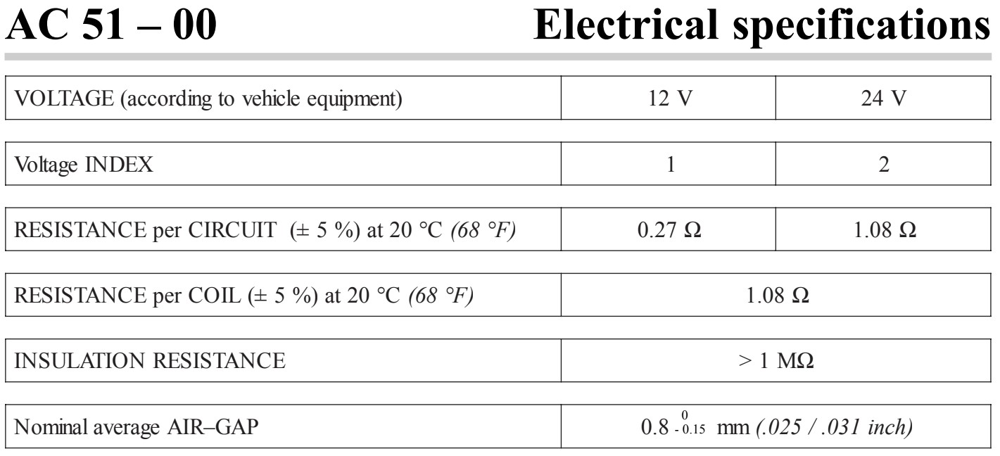 Electrical Specifications
As shown in the datasheet, this brake operates at 12V or 24V. This compatibility reflects its intended application as a retarder for commercial trucks, which typically rely on these standard battery systems.
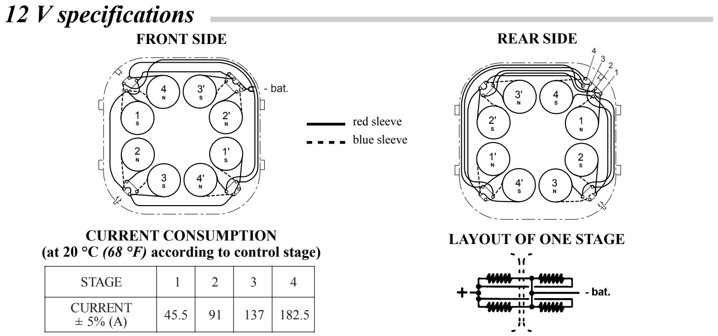 12V Specifications
In the 12V specification all the coils are in parallel (16 total coils, 4 coils in parallel per stage) and in the 24V specification we have two coils in series per stage and two in parallel (8 parallel branches, 2 coils in series each).
Eddy current brakes used in trucks are typically designed with multiple discrete braking stages, in this case four. Each stage corresponds to a predefined level of braking force that the driver can progressively engage.
When the retarder is installed on the truck, the driver selects the desired braking level by activating one or more stages. Engaging the first stage provides a low level of braking force. As additional stages are activated (second, third, and fourth), the braking effect increases incrementally.
Electrically, each stage enables an additional parallel branch within the retarder’s circuit. This increases the total current flowing through the system, which in turn strengthens the magnetic field generated by the retarder. A stronger magnetic field induces higher eddy currents in the rotor, resulting in greater opposing torque and therefore more braking force.
In summary, the staged design allows for controlled, stepwise adjustment of braking force by increasing current through the activation of parallel circuit branches. For my application, this was not the proper way to control the brake.
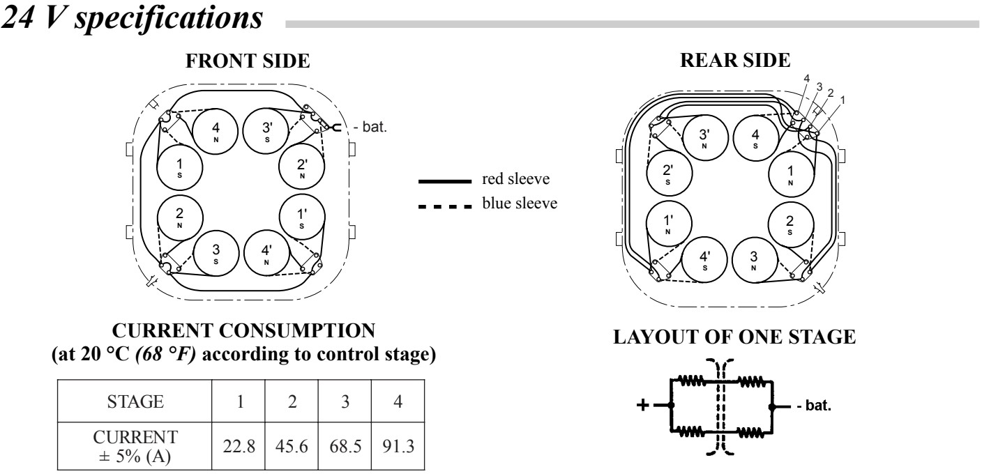 24V Specifications
As we can see In these specifications, if the coils are connected at 12V, the maximum current that the brake can handle is 182A.
If we power it at 24V, the maximum current is 91A. Remember that this is to handle around 1000 Nm and 500 HP. Of course for my purpose I didn’t need that huge amount of power and current but I wanted to have it available in the future.
Handling these amounts of current was not an option. It was going to be difficult to handle it with precision.
Eddy Current Brake Wiring
Finding a controllable power supply capable of delivering 180A at 12V or 90A at 24V is “expensive”. Beyond the cost of the supply itself the power stage electronics required to switch such high currents are difficult to design and prone to failure. In engineering it is almost always more efficient to handle slightly higher voltages rather than current to reduce resistive losses and heat dissipation.
Looking at the electrical specifications each coil has a resistance of approximately 1.08 Ohms. The brake contains a total of 16 coils with 8 located on each side. By default the unit was configured for 12-24V operation with groups of coils in a series-parallel arrangement that simply did not allow for higher voltage inputs. To make the system compatible with higher voltage, a complete rewiring of the internal connections was necessary.
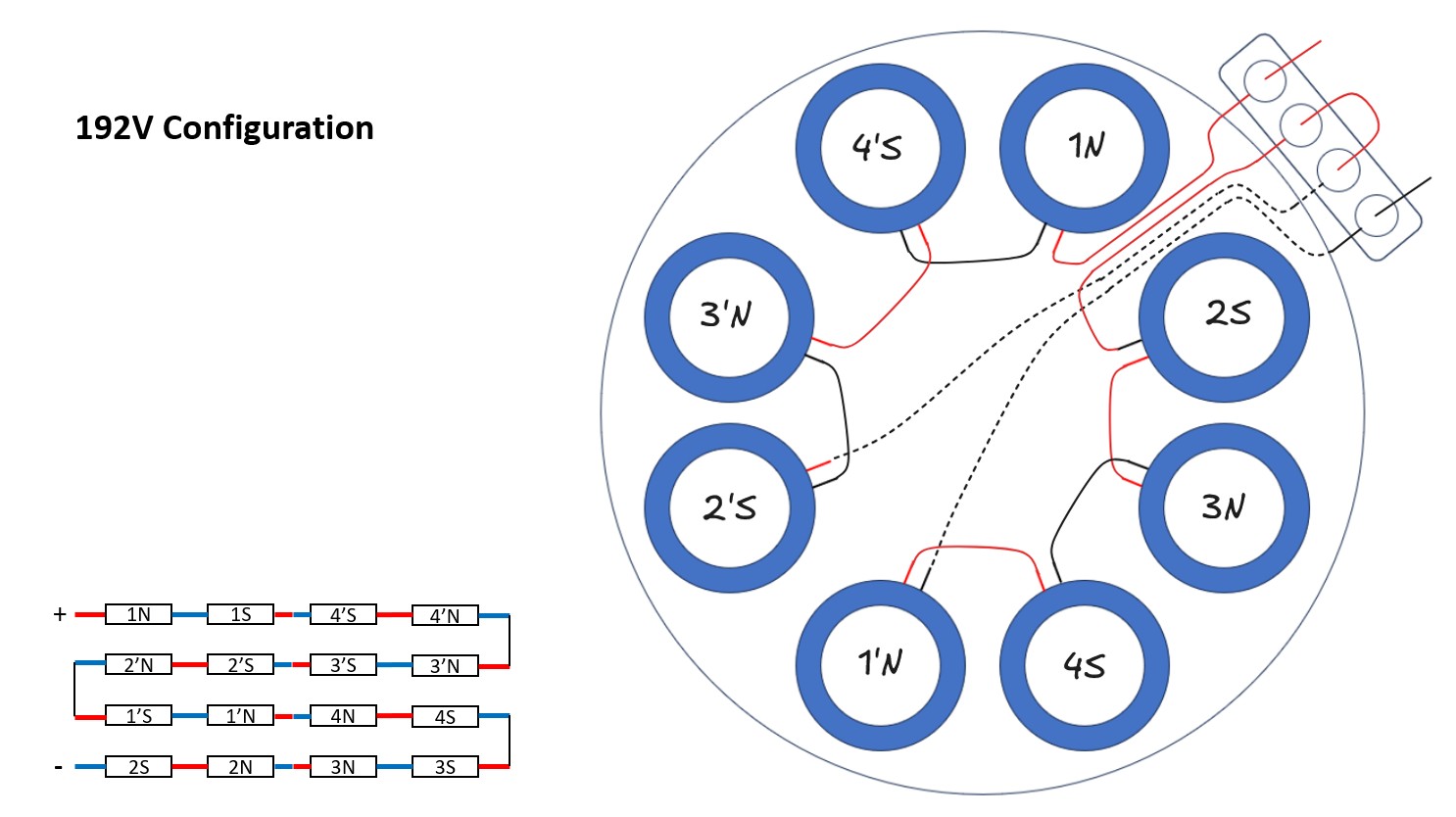 192V Wiring
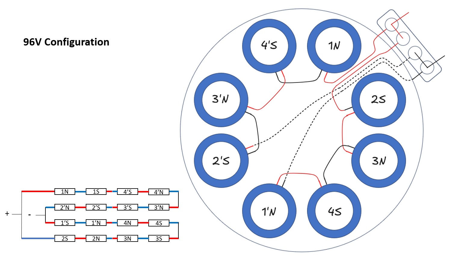 96V Wiring
As shown in the diagrams these new connections allow me to power the electric brake with either 96V or 192V depending on whether the two main branches are connected in parallel or in series. Switching between these configurations is very straightforward using the original terminal block of the brake. By simply moving the jumpers I can adapt the hardware to the available voltage source.
Using higher voltage significantly reduces the required current. Each individual coil is rated for 12V and about 10A maximum. In this new configuration I can achieve the full braking torque of 1000 Nm and handle up to 500 HP using 192V while only drawing about 10A. This makes the power electronics much smaller and more reliable since I no longer have to manage the heat generated by massive current flow.
12V Configuration
We are going to calculate the maximum current we would need to supply to the brake if we worked at 12V:
\[I_{branch} = \frac{V}{R}\] \[I_{branch} = \frac{12 \text{ V}}{1.08 \Omega }\] \[I_{branch} = 11.11 \text{ A}\]With 16 branches in parallel, the total current is:
\[I_{total} = I_{branch} \cdot n\] \[I_{total} = 11.11 \text{ A} \cdot 16\] \[I_{total} = 177.76 \text{ A}\]As we can observe, this result is very close to the 182.5A specified in the manufacturer’s datasheet.
Total Power
To determine the total power of the system, we multiply the voltage by the total current:
\[P_{total} = V \cdot I_{total}\] \[P_{total} = 12 \text{ V} \cdot 177.76 \text{ A}\] \[P_{total} = 2133.12 \text{ W}\]24V Configuration
Let’s calculate the current in the 24V configuration. First, we calculate the resistance of each branch ($R_{branch}$):
\[R_{branch} = 1.08 \Omega \cdot 2 = 2.16 \Omega\]Then, the current per branch:
\[I_{branch} = \frac{V}{R_{branch}}\] \[I_{branch} = \frac{24 \text{ V}}{2.16 \Omega }\] \[I_{branch} = 11.11 \text{ A}\]With 8 branches in parallel (because we have now 2 coils in series on each branch), the total current is:
\[I_{total} = I_{branch} \cdot n\] \[I_{total} = 11.11 \text{ A} \cdot 8\] \[I_{total} = 88.88 \text{ A}\]Total Power
To determine the total power of the system, we multiply the voltage by the total current:
\[P_{total} = V \cdot I_{total}\] \[P_{total} = 24 \text{ V} \cdot 88.88 \text{ A}\] \[P_{total} = 2133.12 \text{ W}\]This was what I was able to do with the default wiring of the eddy current brake. As the current is still a bit high, let’s compare it with the new wiring.
96V Configuration
First, we calculate the resistance of each branch ($R_{branch}$):
\[R_{branch} = 1.08 \Omega \cdot 8 = 8.64 \Omega\]Then, the current per branch:
\[I_{branch} = \frac{V}{R_{branch}}\] \[I_{branch} = \frac{96 \text{ V}}{8.64 \Omega }\] \[I_{branch} = 11.11 \text{ A}\]With 2 branches in parallel, the total current is:
\[I_{total} = I_{branch} \cdot n\] \[I_{total} = 11.11 \text{ A} \cdot 2\] \[I_{total} = 22.22 \text{ A}\]Total Power
To determine the total power of the system, we multiply the voltage by the total current:
\[P_{total} = V \cdot I_{total}\] \[P_{total} = 96 \text{ V} \cdot 22.22 \text{ A}\] \[P_{total} = 2133.12 \text{ W}\]192V Configuration
First, we calculate the resistance of the entire branch ($R_{branch}$):
\[R_{branch} = 1.08 \Omega \cdot 16 = 17.28 \Omega\]Then, the current for the branch:
\[I_{branch} = \frac{V}{R_{branch}}\] \[I_{branch} = \frac{192 \text{ V}}{17.28 \Omega }\] \[I_{branch} = 11.11 \text{ A}\]With only 1 branch, the total current is:
\[I_{total} = I_{branch} \cdot 1\] \[I_{total} = 11.11 \text{ A}\]Total Power
To determine the total power of the system, we multiply the voltage by the total current:
\[P_{total} = V \cdot I_{total}\] \[P_{total} = 192 \text{ V} \cdot 11.11 \text{ A}\] \[P_{total} = 2133.12 \text{ W}\]As we can see, the total power consumption is the same but in one case we use more voltage to get the same power and on the other side we use more current with less voltage to get the same power.
Coil Configurations Summary
| Voltage | Coil Arrangement | Total Current | Total Power |
|---|---|---|---|
| 12V | 16 parallel branches (1 coil per branch) | 177.76 A | 2133 W |
| 24V | 8 parallel branches (2 coils in series) | 88.88 A | 2133 W |
| 96V | 2 parallel branches (8 coils in series) | 22.22 A | 2133 W |
| 192V | 1 parallel branch (16 coils in series) | 11.11 A | 2133 W |
As you configure the coils in series and increase the voltage, the total power dissipation remains constant at 2133 W. However, the total current drops significantly, which allows for thinner wiring and more manageable power electronics (MOSFETs) at higher voltages.
As mentioned previously, my intention was to use a higher voltage with a lower current. Current makes components hot and needs more material but voltage only needs more isolation material.
Eddy Current Brake Control
As we discussed earlier, the brake is now configured to operate at 192V with a current limit of roughly 10A. Managing 192V at 10A is technically much simpler than dealing with 12V at 180A.
The eddy current brake requires a DC current to work. To provide this, I essentially had two main options:
- Battery Power: Using a high-voltage battery pack.
- AC-DC Power Supply: Converting standard mains electricity to the required DC voltage.
I ruled out using a battery pack because I did not want to deal with the constant cycle of charging and monitoring the state of charge during testing. It adds another layer of maintenance that I wanted to avoid for this project.
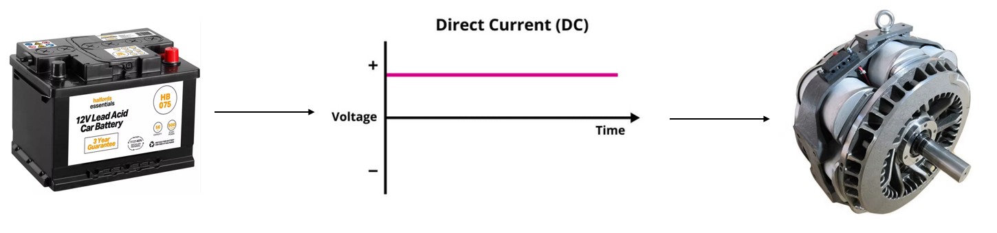 DC-DC Control Concept
Since the power from a standard wall outlet is 230V AC, I needed a conversion stage to transform it into the DC required by the coils.
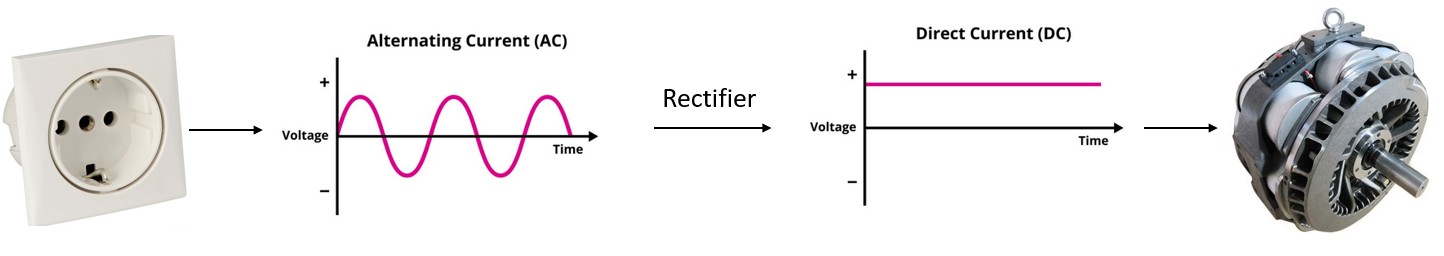 AC-DC Control Concept
Based on the project requirements, the system needed to run on 230VAC at 50Hz, so the AC-DC approach was the way to go.
I looked into commercial power supplies that could hit these voltage and current targets, but I ran into a major problem: response speed.
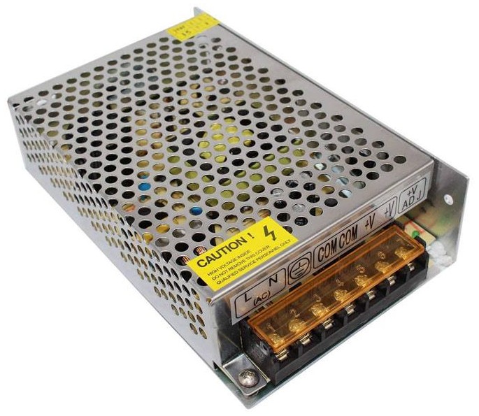 Power Supply
Normally these power supplies have 2 stages. One from, for example, 230VAC to 48VDC and 20A, and another stage for regulating the voltage and current requested by the user. I could use a commercial “first stage” but I would still need to build the second stage.
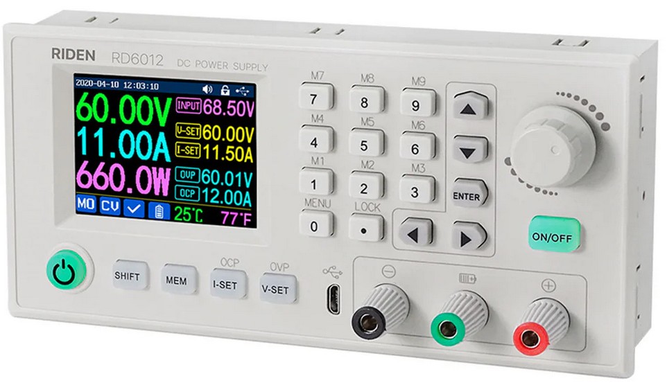 Power Supply - Regulator Stage - Front View
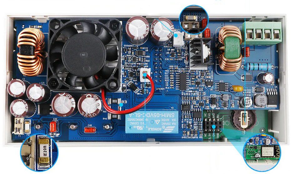 Power Supply - Regulator Stage - Back View
I had no way of knowing how fast these “second stage” could adapt to changes. Specifically, I was worried about the propagation delay between requesting a change in voltage or current and that change actually taking effect at the brake. Most of the commercial units I found relied on communication protocols like RS232 or RS485, which are often too slow for the high-frequency real-time adjustments needed in a dyno control loop. Because of this, I decided that I had to design and build my own custom power stage for this application.
DynoPower
General Requirements
After rewiring the eddy current brake, it can now handle up to 192V and around 10A of peak as mentioned previously. To supply the eddy current brake with DC, I needed to convert AC to DC as seen in the previous image.
To do that I can use a bridge rectifier. Placing the diodes in the following position we are able to get only positive voltage. Thankfully, there are commercial components with the bridge rectifier built inside so it’s easy to implement it. This component has 4 pins. Two of them for the AC side and other two for the DC side. It doesn’t matter which way the AC connections are made but in the DC side we need to take care about because it has polarity.
Polarity: AC vs DC
It is important to distinguish between the two types of electricity here. AC (Alternating Current), like the power from your wall outlet. It does not have fixed polarity, instead, the current periodically reverses direction (50 or 60 times per second). In AC wiring, we talk about Phase (Live) and Neutral rather than positive and negative, as the “positive” side is constantly swapping places with the “negative” side.
In contrast, DC (Direct Current) has a fixed polarity. It has a dedicated Positive (+) terminal and a Negative (-) terminal, and the current always flows in one direction. The bridge rectifier’s job is essentially to take those “swapping” AC inputs and redirect them so they always exit through the same pins, creating a stable (pulsing) positive and negative DC output.
 Bridge Rectifier with Input and Output Signals4
As can be seen in the animation the bridge rectifier uses 4 diodes. When the positive side of the input AC signal goes into it, it allows it to flow. When the negative side of the input signal flows, it reverses the output so also a positive signal is generated in the output.
Another important point is the output quality of the signal. Let’s dive into it in a simplified way.
As we have seen, the AC signal is a sinusoidal signal that crosses the 0V. If we only use a bridge rectifier, we will get a rippled signal like the following one:
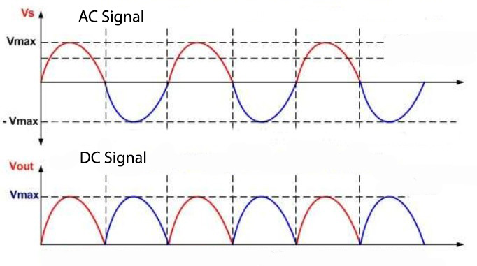 Bridge Rectifier with Input and Output Signals
This presents several problems. One of them is that there is an oscillation that drops to 0V, meaning the result would be exactly as if we were turning the component connected to the rectifier bridge on and off very fast.
Furthermore, in our specific case, this could mean that the eddy current brake’s holding force is not constant. It would generate small peaks of stronger braking followed by valleys of weaker braking, which can cause a sort of mechanical vibration throughout the dynamometer chassis. Naturally, this would severely corrupt the load cell readings, among other issues. The frequency at which this oscillation happens is 100Hz (a 50Hz AC mains frequency becomes 100Hz when full-wave rectified), meaning a complete cycle occurs every 10 milliseconds.
Generally, power supplies use filter circuits made up of capacitors and inductors to solve this. When placed in parallel with the load, a large smoothing capacitor acts like an energy reservoir. It charges up to the maximum voltage during the peak of the AC wave, and when the voltage starts to drop towards 0V, the capacitor discharges its stored energy into the brake, “filling in the gaps” and keeping the voltage much more stable.
With this, we achieve an effect similar to what we can see below:
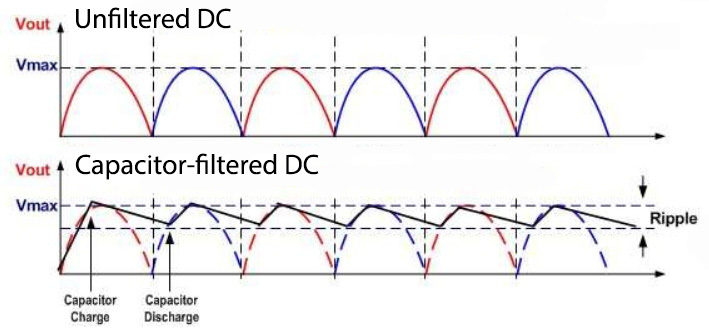 Bridge Rectifier without and with Capacitor
In our specific case, however, introducing massive capacitors and complex filters would unnecessarily complicate the board design, increase the cost and take up a lot of physical space. And not only that, it actually isn’t strictly necessary, as we will see below.
Inductance
While a capacitor resists changes in voltage (by storing energy in an electric field), a coil resists changes in current (by storing energy in a magnetic field).
If the external voltage suddenly drops to zero, the magnetic field inside the coil begins to collapse. This collapse acts like a temporary battery, pushing current forward to keep it flowing steadily. The larger the coil, the higher its Inductance ($L$), and the stronger this current-smoothing effect becomes.
Although the eddy current brake is being fed by a highly rippled pulsing voltage signal, there is a fundamental physical characteristic of its internal coils that plays heavily in our favor here (though it will work against us in another scenario we’ll discuss later). These coils have high inductance.
This means that even though we apply a rapidly fluctuating voltage across them, the current is physically prevented from changing that fast. The inductance forces the current to lag behind the voltage, acting as its own mechanical-electrical filter:
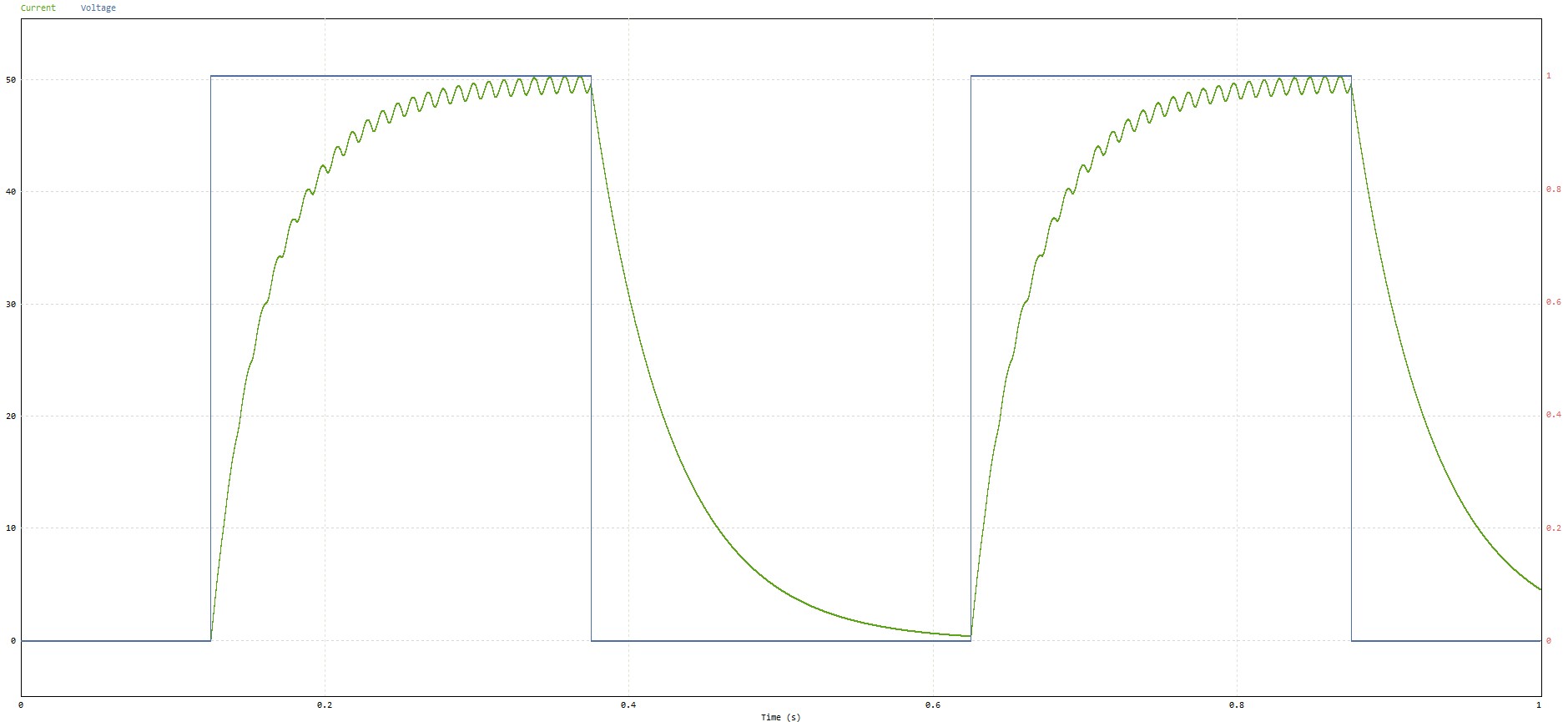 Voltage and Current Applied to a Coil
As can be observed, even though the applied voltage drops to zero or to the high voltage, the current flowing through the coil (and consequently, the braking magnetic field it generates) experiences a natural delay during both its rise and fall. This inherent property is exactly what prevents the power supply’s 100Hz voltage ripple from affecting our braking torque. We could say that the massive coils of the eddy current brake actually act as the final filtering component of our power supply.
Furthermore, as we will see in the next section, we are going to modulate this voltage using PWM (Pulse Width Modulation) at a higher speed than the 100Hz mains ripple. Because the switching frequency (kHz) is fast, the inductor’s time constant ($\tau = L/R$) will easily smooth out the current into a practically flat, steady DC line. Even so, I have still included some small film capacitors in the power system to absorb sharp transient spikes and help keep high-frequency noise (EMI) in check.
With this rectifier element, we have fulfilled one of the primary requirements: converting the AC mains into a usable DC signal. But if we were to input this raw uncontrolled 325V DC directly into the eddy current brake right now, it would draw maximum current, lock the dyno up violently and likely burn out its coils. We need a way to control that power.
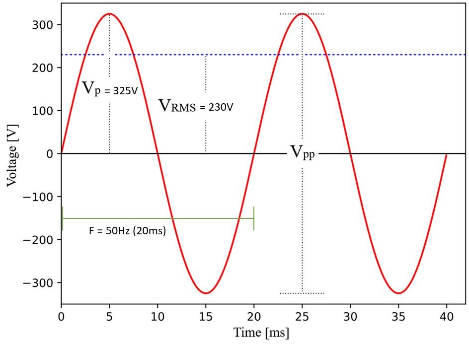 AC Peak and RMS Voltages
We need to understand that when we talk about 230VAC (wall socket voltage), we talk about RMS voltage. In the image we can see a 230VAC signal at 50Hz. The peak voltage is 325V. This means that, after rectified, we will have a DC signal with a maximum of 325V.
If we supply the eddy current brake with 325V directly in the 192V configuration:
Keeping the total branch resistance calculated previously ($R_{branch} = 17.28 \Omega$), we calculate the new current:
\[I_{branch} = \frac{V}{R_{branch}}\] \[I_{branch} = \frac{325 \text{ V}}{17.28 \Omega }\] \[I_{branch} = 18.81 \text{ A}\]Since there is only one branch (all coils in series), the total current is the same:
\[I_{total} = 18.81 \text{ A}\]Total Power
To determine the energy consumption under this new voltage:
\[P_{total} = V \cdot I_{total}\] \[P_{total} = 325 \text{ V} \cdot 18.81 \text{ A}\] \[P_{total} = 6113.25 \text{ W}\]As we can see, if we apply that voltage continuously (the raw 325V DC), around 18 Amps would flow through each coil. This is almost double the maximum current the windings can handle before overheating and burning out.
However, since we are going to modulate the voltage using PWM (Pulse Width Modulation), we don’t need a massive transformer to step down the voltage. All we need to do is introduce a safety limit in the software (and even better if it were in hardware.). Given that the average current is proportional to the pulse width ($I_{avg} = \frac{V_{max} \cdot \text{DutyCycle}}{\text{Resistance}}$), we will configure the microcontroller so that the duty cycle never exceeds a pre-calculated maximum percentage. This way, we limit the maximum current to stay well below the manufacturer’s limit, no matter what happens.
Another critical factor to consider when working with these voltages is dielectric isolation. I had to ensure that the protective enamel on the copper coil wires and the overall insulation relative to the brake chassis were capable of withstanding peaks of over 300V without arcing or shorting to ground. Fortunately, after reviewing the specifications and testing it, my brake’s insulation was more than sufficient.
With all this physical and safety information clear, I finally proceeded with the definitive designs of the power stage.
Design 1 - Thyristor (DynoPower v1)
The first and simplest option I considered was using thyristors.
What is a Thyristor (SCR)?
A Thyristor, often called a Silicon Controlled Rectifier (SCR), is a solid-state semiconductor device that acts as a “latching” switch. Unlike a standard transistor (which requires a continuous signal to stay on), a thyristor only needs a short pulse at its gate terminal to start conducting current from the Anode to the Cathode.
Once it is “fired” (turned on), it stays on indefinitely, even if you remove the gate signal. The only way to turn it off is through a process called commutation, which happens when the current flowing through it drops below a specific “holding” threshold (effectively zero). In AC circuits, this happens naturally every time the sine wave crosses 0V, making thyristors very popular for high-power phase control applications.
There are semi-controlled thyristor modules on the market like the one shown below. These modules take a direct 230V AC input and output a modulated power signal. They offer several control methods, such as using an analog 0-5V or 0-10V signal, or a PWM signal where you vary the duty cycle.
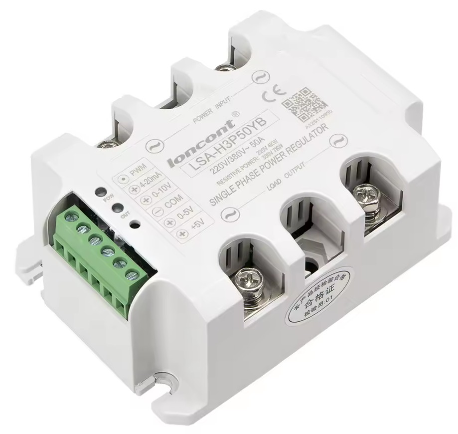 Commercial SCR Module
The idea was for the SCR module to control the amount of energy reaching the eddy current brake. Once the voltage was modulated, I would use a bridge rectifier to convert the signal into DC current. This system does not generate a perfectly smooth DC current as seen previously but it’s valid for the application.
Below is a conceptual schematic of this setup.
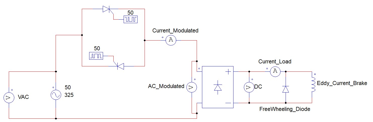 Thyristor Schematic
First, we have a 230V 50Hz AC signal. After passing through the thyristor module, we can modulate that signal to a much smaller percentage while still having positive and negative components. After the bridge rectifier, we get the final signal, a pulsating positive DC current.
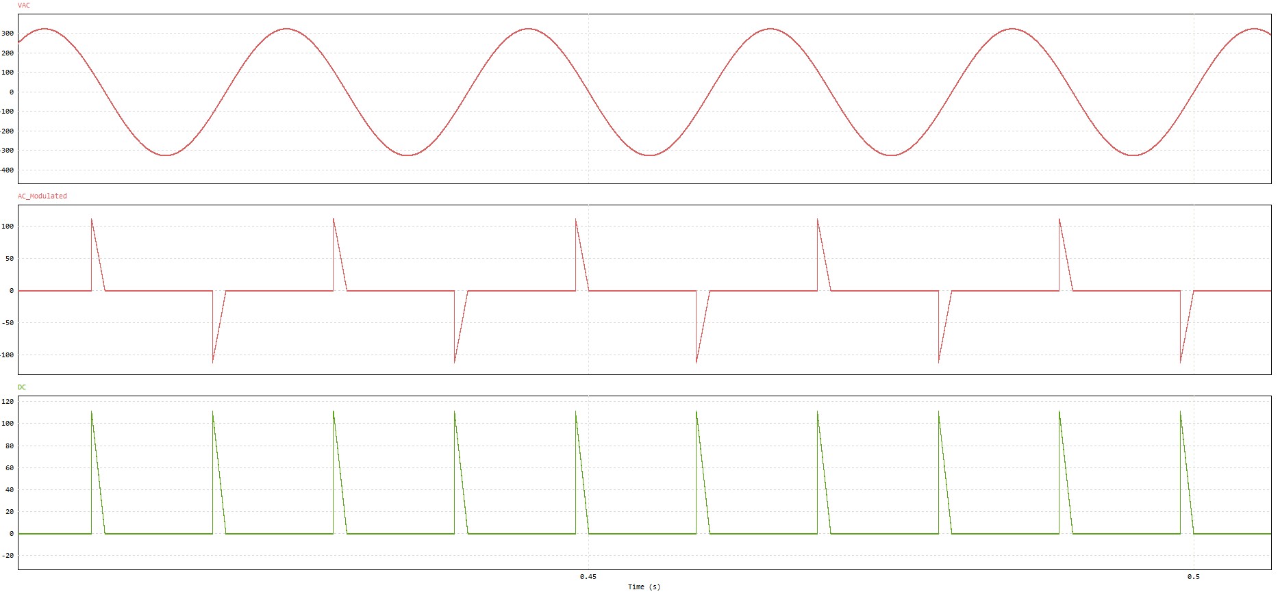 Thyristor Signals at 20% Load
The graph above shows an example with relatively low modulation (20%). As we increase the power, we get a signal closer to the one below, which represents roughly 50% power delivery. The first graph shows the AC signal, the second one the modulated signal by the thyristor and the last one the resulting signal after the bridge rectifier.
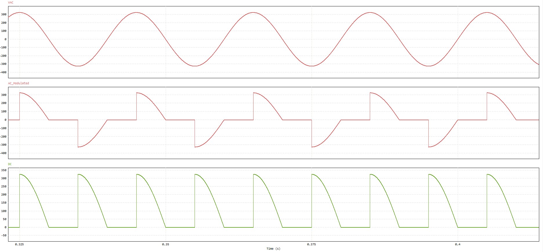 Thyristor Signals at 50% load
As mentioned previously, the capacitors and the coil inductance smooth this signal, preventing those sharp peaks from affecting the braking force too much. However, it is important to understand how a thyristor actually works. To put it simply, unlike a relay, IGBT, or MOSFET, we can tell a thyristor when to turn on (the firing point), but it will not turn off until the current flowing through it drops to near zero.
This means we are strictly limited by the grid frequency (50Hz in Europe) to modulate the voltage. In practice, if I want to make a change, I might have to wait up to 10ms for that change to physically happen. For example:
At $T_0$ (milliseconds), the AC signal passes through 0V. If I decide to trigger the thyristor at $T_5$ (5ms later), it will conduct from $T_5$ until $T_{10}$ (the next zero crossing). If at $T_{27}$ the control system decides it needs less current, the thyristor cannot update its state until the next cycle at $T_{35}$ or later. In the worst-case scenario, there is a 10ms delay before the hardware reacts.
With this design ready I manufactured the PCB and soldered all the components:
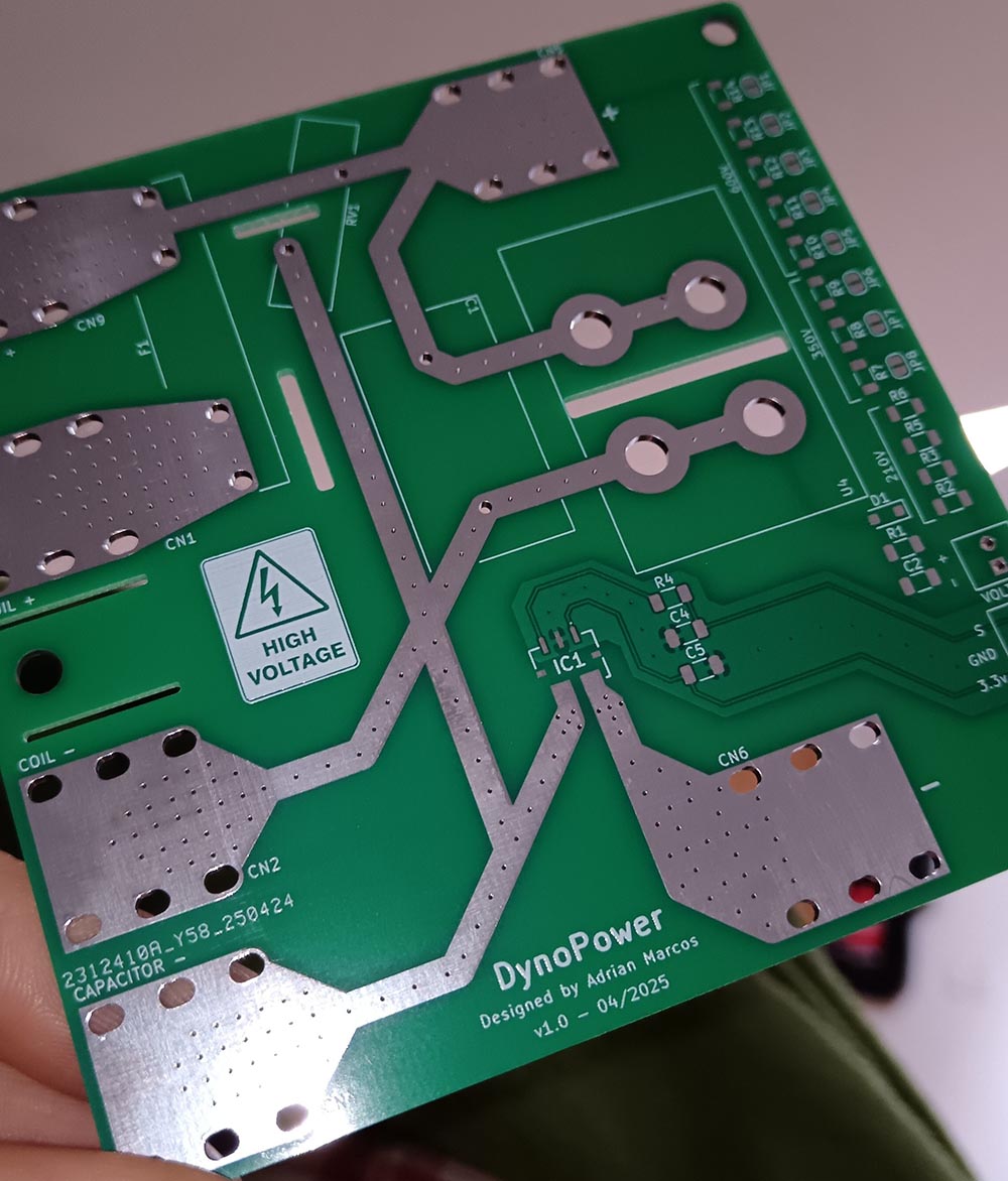 DynoPower V1 PCB
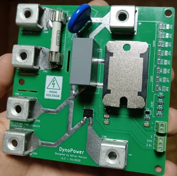 DynoPower V1 PCB with Components
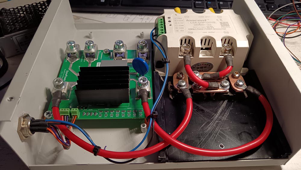 DynoPower V1 + Bridge Rectifier + Thyristor Module
Unfortunately, I lost a lot of time diagnosing a problem with this design. After a detailed analysis, I realized the commercial module was not as fast as I expected. I did not measure the exact internal delay, but it was certainly much higher than 10ms from the moment the command was sent until the thyristor actually reacted. This is likely because the module has its own internal filtering electronics that are not optimized for high-speed real-time response.
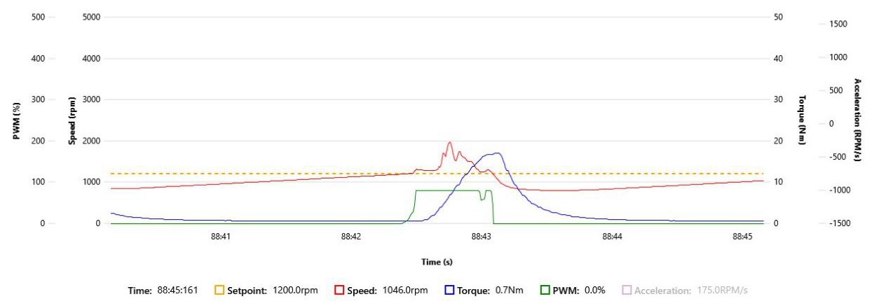 Thyristor Delay
As you can see in the graph, there is almost half a second of delay between the command signal (green line) and the response reflected by the load cell (blue line). The only relatively fast response occurred when the PWM signal dropped to zero, but even then, it was far too slow for the precision and responsiveness I was looking for.
I later found that companies like Semikron offer specialized modules (SEMIKRON RT380M B2HKF Datasheet) that would likely work perfectly, but they are quite expensive and I would still be fighting the inherent 10ms limitation of the 50Hz grid. With the thyristor option discarded, I moved on to faster alternatives.
Design 2 - SiC MOSFET with Free-Wheeling Diode
In the previous design I used a thyristor to modulate the current. At that time I had no experience with this type of power electronics. I realized I needed a MOSFET or something similar to modulate the current more effectively. The new strategy was to first rectify the AC current into DC and then modulate it.
For reasons I cannot quite remember now I decided to try using a SiC MOSFET. This is a type of MOSFET that supports relatively high currents, is very fast, and has very low switching losses. However I later realized that this technology was too good for two main reasons:
- Operating Frequency: SiC MOSFETs are designed for very high-speed applications. My project only required a frequency between 1 and 4 kHz which is well within the range of much cheaper components like IGBTs.
- Switching Speed ($dv/dt$): The switching is so fast that it creates a very high $dV/dt$. While this is an advantage at high frequencies it was a disadvantage here because such rapid changes produce significant Electromagnetic Interference (EMI).
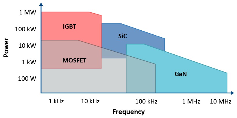 Power and Frequency of IGBT, SiC, MOSFET and GaN5
As seen in the graph, IGBTs are the components that support the highest power but operate at lower frequencies. Even so they easily cover my 1-4 kHz range. Similarly, SiC MOSFETs support relatively high currents and much higher working frequencies but it was simply too much for this application.
Due to some initial misconceptions I thought a single SiC MOSFET would not be enough to handle the current and that I would need to use two in parallel. Since I was not entirely familiar with how these components behaved in parallel I decided to manufacture two test PCBs with different gate drivers and configurations which I will analyze in detail below.
Testing Different Gate Drivers
The initial idea for this board was to be able to use two SiC MOSFETs in parallel and test the different configurations and features of various gate drivers. This was primarily because SiC MOSFETs generally handle a bit less current than traditional high-power IGBTs and I had also initially made some erroneous calculations regarding the maximum current consumption of the eddy current brake.
Finally, I didn’t physically test every single configuration because I realized that using two SiC MOSFETs in parallel wasn’t actually necessary for my current load. Even so, I am going to proceed analyzing the initial design idea in detail.
We need to be clear on a few key concepts before diving into these designs:
- Isolated Drivers: All the drivers we are going to use are galvanically isolated. This means that the low-voltage control side (the PWM signal from the microcontroller) is electrically separated from the high-voltage “power” side (the MOSFET gate). This protects our logic board from high-voltage spikes and short circuits.
- $dV/dt$ (Rate of Voltage Change): This represents how fast the voltage transitions from one level to another when a MOSFET switches. Because SiC chips are so fast, the drain voltage can shoot from 0V to 325V in nanoseconds. According to the law ($I = C \cdot \frac{dV}{dt}$), this extreme voltage change forces a physical current backward through the MOSFET’s internal parasitic capacitance (the Miller capacitance) and injects it directly into the gate.
- Active Miller Clamp (MC): This feature directly combats the dangers of high $dV/dt$. If the parasitic current injected into the gate is strong enough, it can charge the gate voltage back up and accidentally turn the MOSFET on while it is supposed to be off (parasitic turn-on). An Active Miller Clamp is a pin on the gate driver that detects when the gate voltage drops below a safe level and internally shorts the gate directly to ground. This holds the MOSFET off, absorbing that parasitic current and preventing false triggers.
- EMI Generation ($dV/dt$): While SiC MOSFETs are fast switching and reducing thermal power losses (heat), that exact same speed is the absolute worst enemy of Electromagnetic Compatibility (EMC). High $dV/dt$ creates two major issues:
- Harmonics: The rapid voltage transitions generate high-frequency harmonics that act like radio waves, radiating noise directly off the PCB traces.
- Common-Mode Noise: The rate of voltage change forces parasitic currents through the tiny capacitances between the MOSFET’s drain and the grounded heatsink. This noise travels through the chassis ground and can easily corrupt delicate sensor readings. This is exactly why I use a larger gate resistor (like the 10 $\Omega$ one mentioned earlier). It intentionally slows down the $dV/dt$, sacrificing a tiny bit of thermal efficiency and speed to keep the electrical noise clean and manageable.
With these concepts clear, I implemented all the configurations that can be seen in the schematic using different drivers:
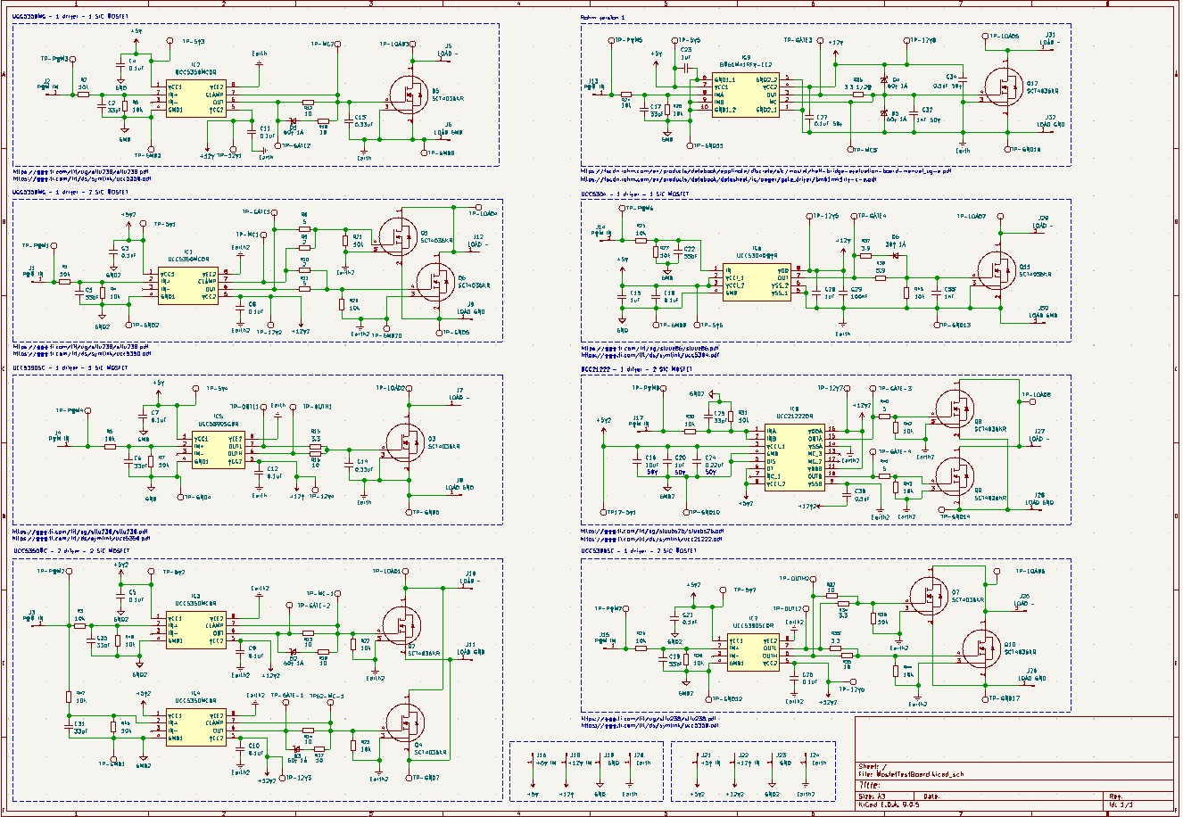 Gate Driver Test Configurations
NOTE: In all the driver PWM inputs, the 10k resistor in series to PWM must be removed. If not, it works as voltage divider with the 10k resistor in parallel.
UCC5350MC - 1 Driver - 1 MOSFET
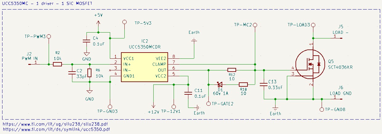 UCC5350MC - 1 Driver - 1 MOSFET
This configuration consists of a single isolated gate driver (UCC5350MC) controlling a SiC MOSFET. The logic side of the driver is powered at 5V while the isolated gate-drive side is typically powered at 15V to 18V (depending on the specific SiC MOSFET’s requirement). It is crucial to remember that the logic ground (GND) and the high-power ground (Earth/Power GND) are completely isolated planes. The driver’s internal galvanic isolation ensures that high-voltage spikes from the power side never reach the logic side. I also added test points to easily probe the input and output signals with an oscilloscope.
To fully understand this schematic, it helps to know what each pin on the UCC5350MC does:
VCC1andGND1provide the power supply for the logic side.IN+is the non-inverting input where our PWM signal enters, whileIN-is the inverting input (tied toGND1so the driver operates in non-inverting mode).- On the other side of the driver,
VCC2andVEE2are the isolated power supply for the gate drive.OUTis the main output pin that pushes current to charge the MOSFET gate. CLAMPis the Active Miller Clamp pin used to prevent accidental turn-ons.
On the logic side, the PWM signal from the microcontroller is connected to the IN+ pin. I included a 10k$\Omega$ pull-down resistor R6 and a 33pF capacitor C2 in parallel with GND. The 10k$\Omega$ resistor acts as a safety pull-down, if the microcontroller resets or the wire disconnects, this ensures the PWM input is forcefully pulled to 0V, keeping the MOSFET safely turned off. The 33pF capacitor acts as a high-frequency noise filter. It absorbs tiny electrical transients or EMI spikes on the logic line, preventing false triggers that could accidentally turn the MOSFET on for a microsecond.
On the output side, there is a 10$\Omega$ gate resistor in series with the OUT pin. The value of this resistor dictates how fast the MOSFET changes states. A larger resistor limits the peak current drawn from the driver and slows down the voltage transition. If we don’t need extremely high-frequency switching (which is my case for an eddy current brake) you can use a slightly larger resistor. It artificially slows down the switching transition which reduces generated EMI.
Because SiC MOSFETs can switch fast, when the drain voltage rises rapidly, it can push current backwards through the MOSFET’s internal parasitic capacitance and into the gate. This can cause the gate voltage to rise unexpectedly and turn the MOSFET back on while it’s supposed to be off. The CLAMP pin solves this. When the driver senses the gate voltage dropping below 2V, the internal clamp activates and shorts the gate directly to VEE2. The diode D1 and resistor R18 on this path allow us to fine-tune the turn-off and clamping behavior independently of the turn-on path, ensuring the MOSFET is pulled low aggressively and stays firmly shut.
You will also notice a capacitor C13 placed very close to the VCC2 and VEE2 pins. Turning on a large SiC MOSFET requires a sudden, massive burst of peak current. The main power supply cannot deliver this fast enough due to trace inductance. C13 acts as a local energy reservoir, providing that instantaneous burst of current directly to the driver exactly when it needs it.
Finally, it is essential to clarify that this circuit operates as a low-side switch. This means we are interrupting the negative (ground) return path of the circuit, not the positive supply. The LOAD- (Drain) connects to the bottom of the load (the eddy current brake coils). Even though it’s labeled “negative” relative to the load, it is the more positive of the two ground-side connections when the MOSFET is off. The LOAD GND (Source) connects to the absolute main power supply ground. When the MOSFET turns on, it bridges LOAD- to LOAD GND, completing the circuit and allowing current to flow from the high-voltage positive supply, through the load, and down to ground.
UCC5350MC - 1 Driver - 2 MOSFET
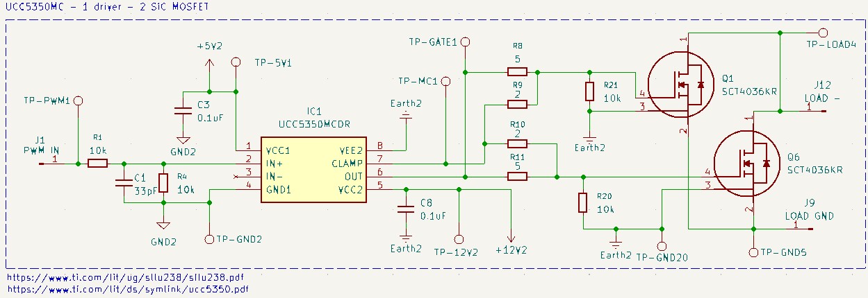 UCC5350MC - 1 Driver - 2 MOSFET
This configuration uses the same isolated gate driver (UCC5350MC) as the previous setup, but it is now configured to control two SiC MOSFETs (Q1 and Q6) in parallel. By paralleling two SCT4036KR SiC MOSFETs, the circuit can handle significantly higher current loads and distribute heat more effectively across the two packages, which is ideal for a larger eddy current brake system. The logic side and high-power side remain completely isolated to protect the controller from high-voltage transients.
The circuit is quite similar to the previous one.
On the output side, the drive signal from the OUT pin (Pin 6) is split through two individual gate resistors, R9 and R10 (2$\Omega$ each). These individual resistors are critical when paralleling MOSFETs because they decouple the gates from one another, preventing parasitic oscillations that can occur if the gates were connected directly. Additionally, I added 10k$\Omega$ gate-to-source resistors (R21 and R20) directly at each SiC MOSFET. These provide a local safety path to ground for each gate, ensuring both devices stay firmly off even if a trace connection back to the driver fails.
UCC5390SC - 1 Driver - 1 MOSFET
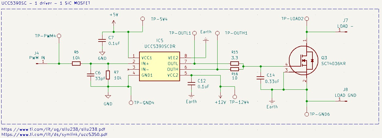 UCC5390SC - 1 Driver - 1 MOSFET
This configuration introduces the UCC5390SC isolated gate driver. While it shares the same galvanic isolation principles as the previous drivers, the “SC” variant features split outputs (OUTH and OUTL). This allows us to independently control the turn-on and turn-off speeds of the SCT4036KR SiC MOSFET, providing finer control over switching losses and EMI.
To understand the specific pinout of the UCC5390SC:
VCC1andGND1provide the 5V power supply for the logic side.IN+andIN-are the PWM input pins (configured in non-inverting mode as previously described).- On the isolated side,
VCC2andVEE2provide the power supply (shown here at +12V). OUTHis the dedicated pin for charging the gate (turn-on).OUTLis the dedicated pin for discharging the gate (turn-off).
On the logic side, the PWM signal enters via J4. Following the design choice from previous configurations, the series resistor (R5) is removed to prevent voltage division, ensuring the IN+ pin receives the full 5V signal. The 10k$\Omega$ pull-down resistor (R7) and the 33pF capacitor (C6) remain in place to provide the same safety pull-down and noise filtration functions discussed in the earlier posts.
The primary advantage of this circuit is the asymmetric gate drive stage. The OUTH pin connects to the gate through a 10$\Omega$ resistor (R16), while the OUTL pin connects through a 3.3$\Omega$ resistor (R15). By using a larger resistor for turn-on and a smaller one for turn-off, we can slow down the initial activation to minimize EMI, while ensuring the MOSFET shuts down extremely fast to reduce switching energy losses and prevent accidental turn-ons.
The power stability on the isolated side is maintained by C12 ($0.1\mu F$) and C14 ($0.33\mu F$). As previously explained, these capacitors act as local energy reservoirs, supplying the high peak currents required to move the gate charge of the SiC MOSFET quickly.
Finally, as the previous designs, this remains a low-side switch configuration.
UCC5350MC - 2 Driver - 2 MOSFET
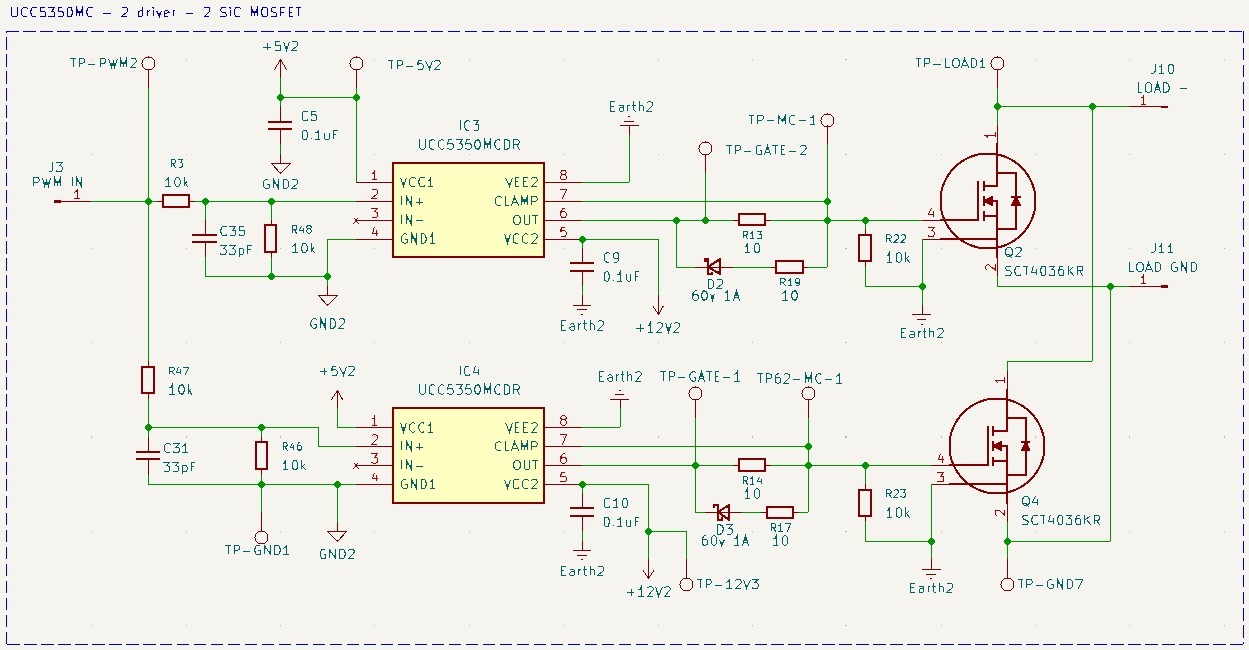 UCC5350MC - 2 Driver - 2 MOSFET
This configuration takes the paralleling concept from the previous UCC5350MC setup a step further. Instead of sharing a single driver across two MOSFETs, here each transistor (Q2 and Q4) gets its own dedicated UCC5350MC (IC3 and IC4). In this “one-driver-per-gate” approach each MOSFET receives its own current source, eliminating any risk of gate-signal weakening or timing skew between the two transistors.
The PWM signal from J3 is split to feed both drivers. As before, the series resistors (R3 and R47) are removed, and each channel retains its own 10k$\Omega$ pull-down (R48, R46) and 33pF filter capacitor (C35, C31). This redundancy ensures both drivers independently filter noise and remain safely off if the control signal is lost.
Each output stage is identical to the single-driver, single-MOSFET design: a 10$\Omega$ gate resistor (R13 for Q2, R14 for Q4) and a dedicated Active Miller Clamp circuit with its own diode (D2/D3) and 10$\Omega$ resistor (R19/R17). By keeping the drive paths entirely separate until the MOSFET gates, we prevent any parasitic interactions or ringing between the two transistors. Individual 10k$\Omega$ gate-to-source pull-downs (R22, R23) are also included at each MOSFET.
The key difference in power delivery is that each driver has its own decoupling capacitor (C9 and C10) on the isolated side. This is important because switching two MOSFETs simultaneously draws double the peak current, and having a dedicated capacitor per driver ensures the voltage rail remains stable during the rapid charging of the gate capacitances.
BM61M41RFV - 1 Driver - 1 MOSFET
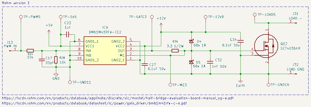 BM61M41RFV - 1 Driver - 1 MOSFET
This configuration introduces the BM61M41RFV-CE2, an isolated gate driver from Rohm. The functional goal is the same as our previous designs, but the pinout and some peripheral choices differ.
The BM61M41RFV pinout:
VCC1andGND1provide the 5V logic-side supply.INAis the primary PWM input, whileINBis tied to ground for non-inverting operation.VCC2andGND2provide the isolated 12V gate-drive supply.OUTis the primary gate-drive output.MCis the Active Miller Clamp pin, functioning identically to theCLAMPpin on the UCC5350MC.
The logic side follows the same established pattern: R24 removed, 10k$\Omega$ pull-down (R28) and 33pF capacitor (C17) retained.
This circuit includes two Schottky clamping diodes (D4 and D5) that clamp the gate voltage to the supply rails, preventing inductive spikes from exceeding the driver’s maximum ratings. A 1nF capacitor (C32) is placed directly between gate and source for additional high-frequency noise damping, a component not present in the previous designs.
On the power side, decoupling is handled by C23 ($1\mu F$) on the logic side, and C27 ($0.1\mu F$) and C34 ($0.1\mu F$) on the isolated side. I extracted this schematic as part of a ROHM’s application note.
UCC5304 - 1 Driver - 1 MOSFET
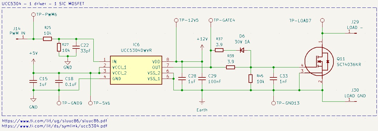 UCC5304 - 1 Driver - 1 MOSFET
This configuration features the UCC5304, a simpler isolated single-channel gate driver. Unlike the UCC5350MC and UCC5390SC, this driver has no Active Miller Clamp pin and only a single output. To compensate, the circuit uses an external diode-resistor network to achieve asymmetrical switching speeds and paths.
The UCC5304DWYR pinout:
INis the PWM input.VCC1andGNDprovide the 5V logic-side supply.VDDprovides the isolated +12V drive supply, whileVSS(Pins 5, 6) connects to the high-power ground.OUTis the single output pin used for both charging and discharging the gate.
The logic side is identical to previous designs: series resistor R25 removed, 10k$\Omega$ pull-down (R27) and 33pF capacitor (C22) retained.
The different part of this circuit is how it achieves asymmetric switching with a single output pin:
- During turn-on,
OUTgoes high and current flows through the 3.9$\Omega$ resistor (R39) to charge the gate. - During turn-off,
OUTgoes low and the gate discharges throughR39in parallel with the series combination of another 3.9$\Omega$ resistor (R37) and a diode (D6). The diode only conducts in the discharge direction, effectively halving the resistance during turn-off.
This makes the MOSFET shut down significantly faster than it turns on, achieving a similar behavior to the UCC5390SC’s split outputs, but using a standard single-output driver.
A 10k$\Omega$ gate-to-source resistor (R45) provides a local safety pull-down, and a 1nF capacitor (C33) suppresses high-frequency oscillations at the gate, similar to the ROHM configuration. Decoupling on the isolated side is handled by C28 ($1\mu F$) and C29 ($100nF$).
UCC21222 - 1 Driver - 2 MOSFET
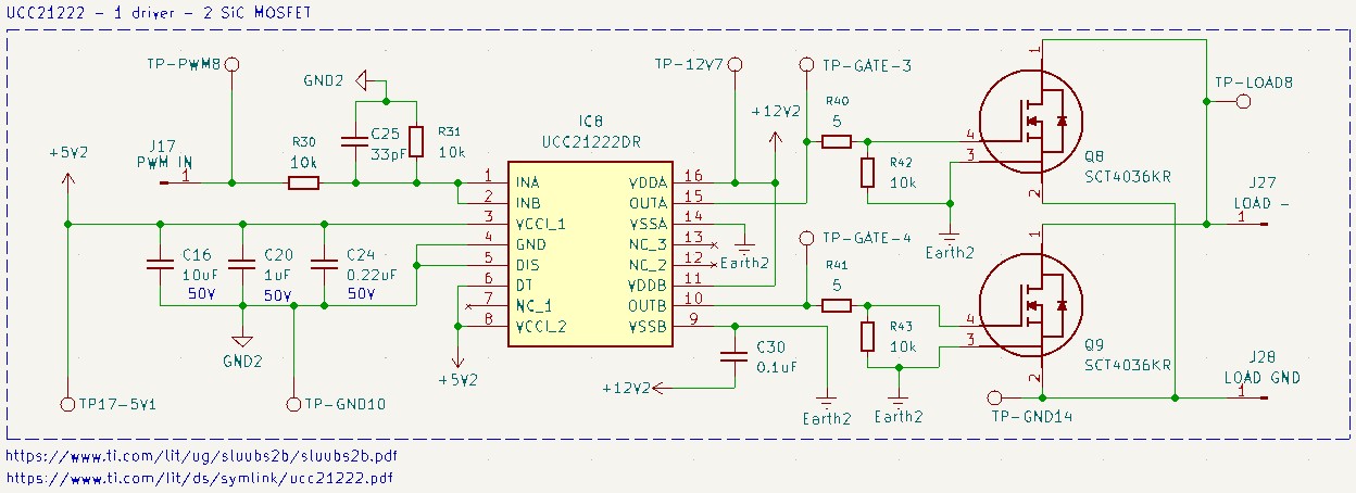 UCC21222 - 1 Driver - 2 MOSFET
This configuration introduces the UCC21222, a dual-channel isolated gate driver, to control two MOSFETs (Q8 and Q9) in parallel. Unlike the earlier UCC5350MC 1-driver-2-MOSFET setup that fanned out a single output to two gates, this IC has two fully independent channels, each with its own output stage. This provides dedicated drive strength and timing for each transistor.
The UCC21222DR pinout:
INAis the PWM input.INBis tied to ground for non-inverting operation.VCCI_1andVCCI_2provide the 5V logic-side supply, whileGNDis the logic ground.DISis a disable pin andDTis a dead-time control pin. Both are tied to ground since we don’t need these features for a simple low-side switch.- On the isolated side,
VDDAandVDDBprovide the +12V isolated drive supplies. OUTAandOUTBare the independent outputs driving each MOSFET gate.VSSAandVSSBconnect to the high-power ground.
The logic-side filtering follows the same pattern: R30 removed, 10k$\Omega$ pull-down (R31) and 33pF capacitor (C25) in place, plus a decoupling network (C16, C20, C24) on the logic supply.
Each MOSFET is driven through its own channel: OUTA drives Q8 through a 5$\Omega$ resistor (R40), and OUTB drives Q9 through an identical 5$\Omega$ resistor (R41). By using the independent channels instead of a shared output, we eliminate gate-to-gate interactions and parasitic oscillations without needing the separate resistor decoupling that was critical in the shared-driver approach. Individual 10k$\Omega$ gate-to-source pull-downs (R42, R43) are included at each MOSFET.
Note that this driver does not include an Active Miller Clamp, so protection against parasitic turn-on relies on the gate resistor values and the 10k$\Omega$ pull-downs keeping the gates firmly at ground potential.
Isolated-side decoupling uses C30 ($0.1\mu F$).
UCC5390SC - 1 Driver - 2 MOSFET
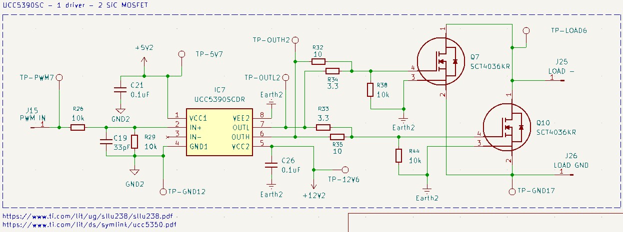 UCC5390SC - 1 Driver - 2 MOSFET
This final configuration extends the single-MOSFET UCC5390SC design to drive two MOSFETs (Q7 and Q10) in parallel, combining the split-output advantage of the UCC5390SC with the current-handling capability of paralleled transistors.
The logic side is identical to the UCC5390SC single SiC MOSFET version: series resistor R26 removed, 10k$\Omega$ pull-down (R29) and 33pF capacitor (C19) retained.
The key change is in the gate drive stage, where each split output now fans out to two gates:
- Turn-on:
OUTHsplits through two 10$\Omega$ resistors (R32andR35), one per MOSFET. The higher resistance slows the turn-on to manage EMI. - Turn-off:
OUTLsplits through two 3.3$\Omega$ resistors (R34andR33), one per MOSFET. The lower resistance ensures both gates discharge quickly, minimizing switching losses and Miller-effect risk.
As with all paralleled-MOSFET designs in this series, dedicated 10k$\Omega$ gate-to-source pull-downs (R38, R44) are placed at each SiC MOSFET for localized safety. The individual resistors on each gate path also serve to decouple the two gates from each other, preventing the parasitic oscillations discussed in the UCC5350MC 1-driver-2-MOSFET configuration.
Isolated-side decoupling uses C26 ($0.1\mu F$).
After that, I manufactured the PCBs to test it:
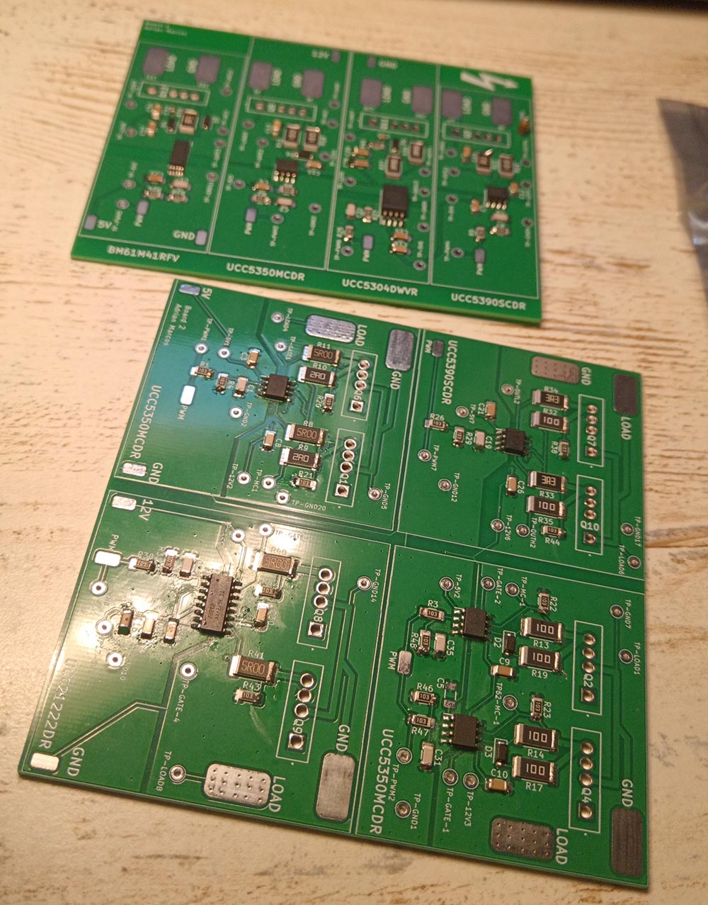 Gate Driver Test PCBs
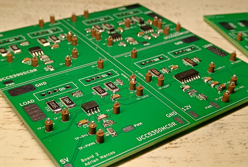 Gate Driver Test PCB
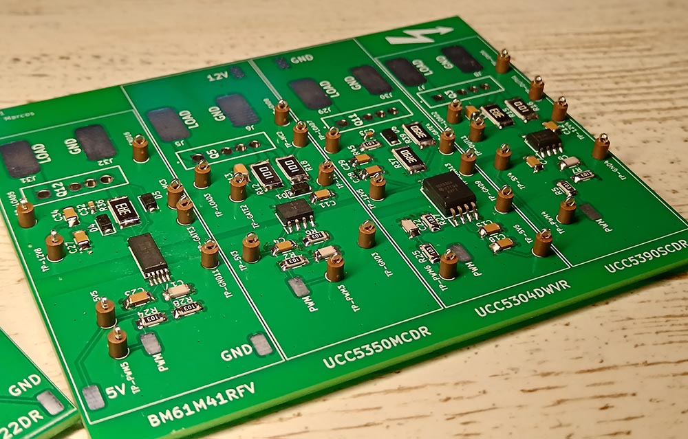 Gate Driver Test PCB
As mentioned previously, I didn’t use a SiC MOSFET for my final design. It was too fast for the application and unnecessary so I moved to an IGBT design.
Gate Drive Voltage
It is essential to ensure that the gate-source voltage ($V_{GS}$) aligns strictly with the datasheet requirements, typically 15V to 18V for these SiC MOSFETs.
At this insufficient voltage, the MOSFET does not reach full enhancement (saturation). This means the internal conductive channel is not fully “open,” resulting in significantly higher on-resistance ($R_{DS(on)}$) than the device is rated for.
Because the resistance is high, the device generates extreme heat. This rapid thermal buildup leads to failure within milliseconds. I burned out two SiC MOSFETs for this reason! I was powering them at 12V instead of 15V!
Design 3 - IGBT with Free-Wheeling Diode (DynoPower v2)
This is the board currently in use
As I mentioned before, using a SiC MOSFET for this application does not make much sense. It is simply too fast.
Even though my tests were successful and the SiC MOSFET board worked perfectly, I decided to switch to an IGBT instead. In general, as we saw earlier, IGBTs can handle higher currents. This meant I no longer needed to mount two components in parallel because a single IGBT was more than enough, which simplified the circuit design. Additionally, an IGBT is typically more robust than a SiC MOSFET when facing unexpected current spikes.
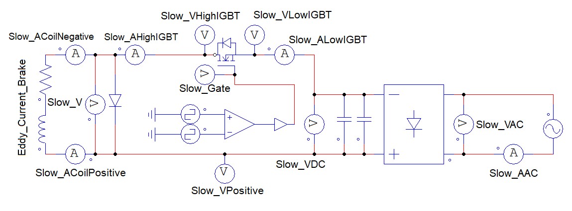 IGBT Schematic
In this simplified schematic you can see how the system operates. On the right side it takes the 230VAC current, passes it through a bridge rectifier and some capacitors to convert it into DC. After that the current flows through the eddy current brake coil. As we can observe the IGBT switches the current on the low side (the negative path). This is an important detail as many people assume these elements switch the positive side but in this configuration they manage the ground return.
After testing several drivers, the one that performed best with the IGBT was the UCC5304DWVR. This is the driver used on DynoPower v2 (the board currently on the dyno). The later v3 redesign switches to the more capable onsemi NCV57001 driver (see Design 3.1 below).
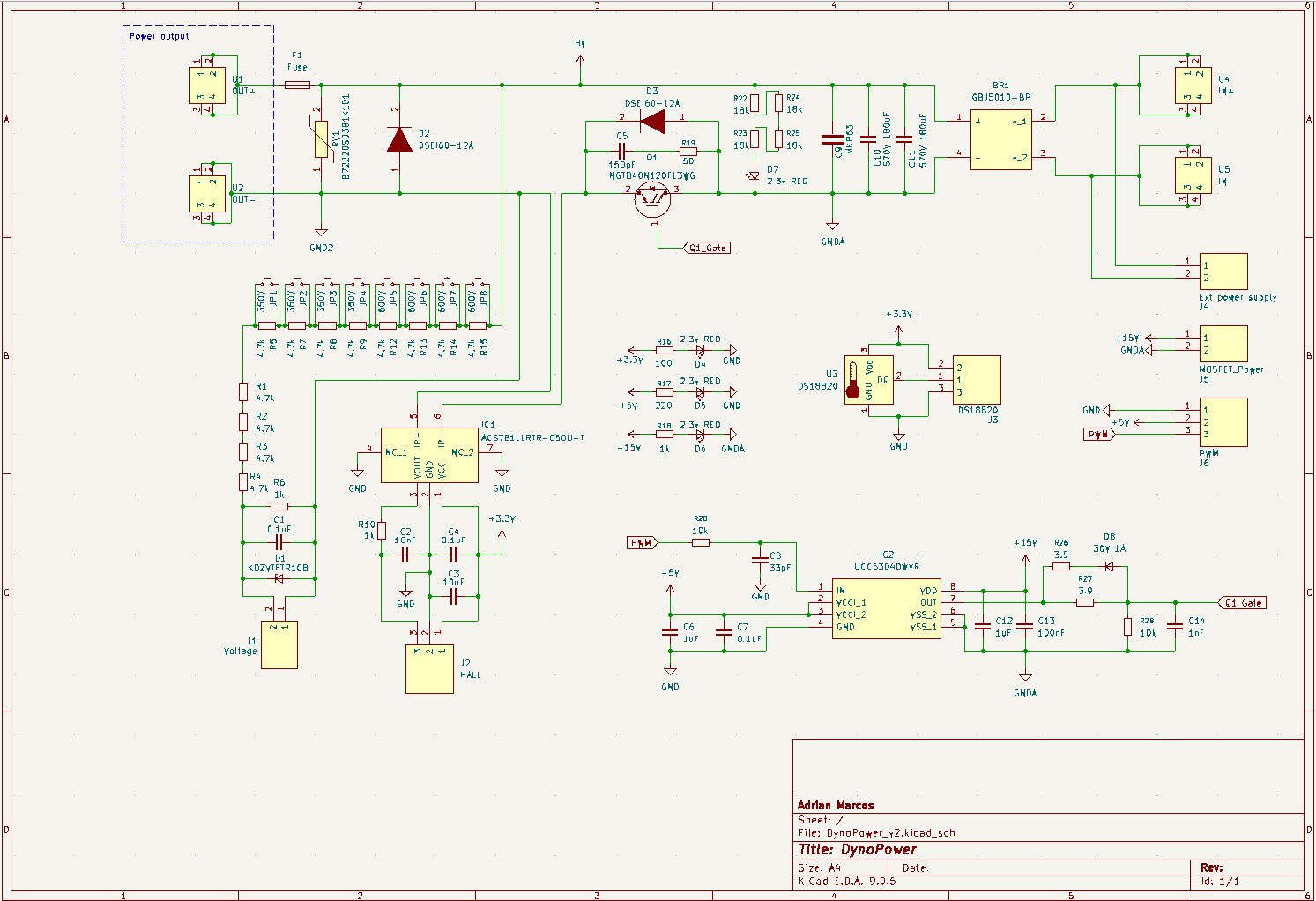 DynoPower V2 Schematic
The schematic is relatively straightforward. Starting from the top left we have the connectors for the 230VAC input. This is followed by a bridge rectifier (GBJ5010). On the rectified DC output I placed three capacitors, two 180uF units and one MKP63. This last one could technically be omitted. Following this there is an indicator LED with a series of resistors that I will explain later.
On the negative side of the circuit you can find the IGBT. This component includes an anti-parallel diode for protection against reverse voltage transients. This is crucial because when the IGBT turns off the magnetic field in the brake coils collapses which can create a massive voltage spike.
Here you can see what happens when the IGBT is conducting:
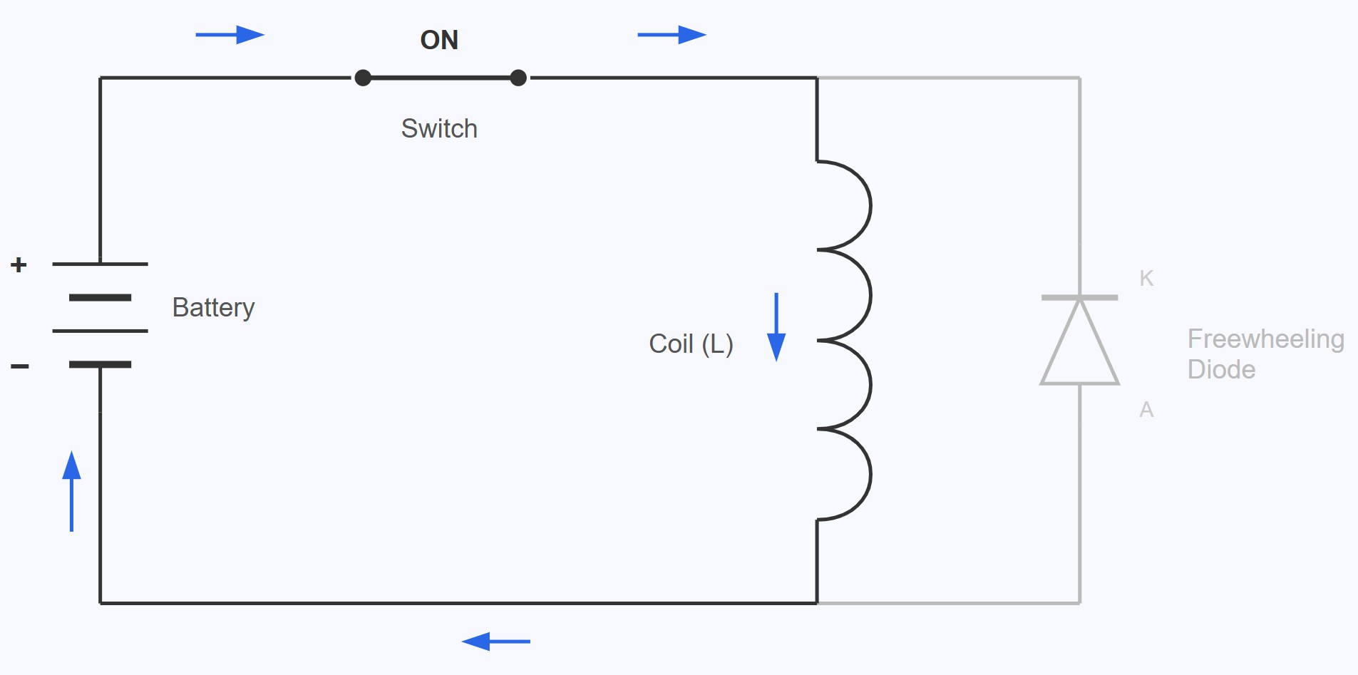 Closed Circuit
In this state, the current flows through the brake coils generating brake torque. The problem appears when the switch is opened.
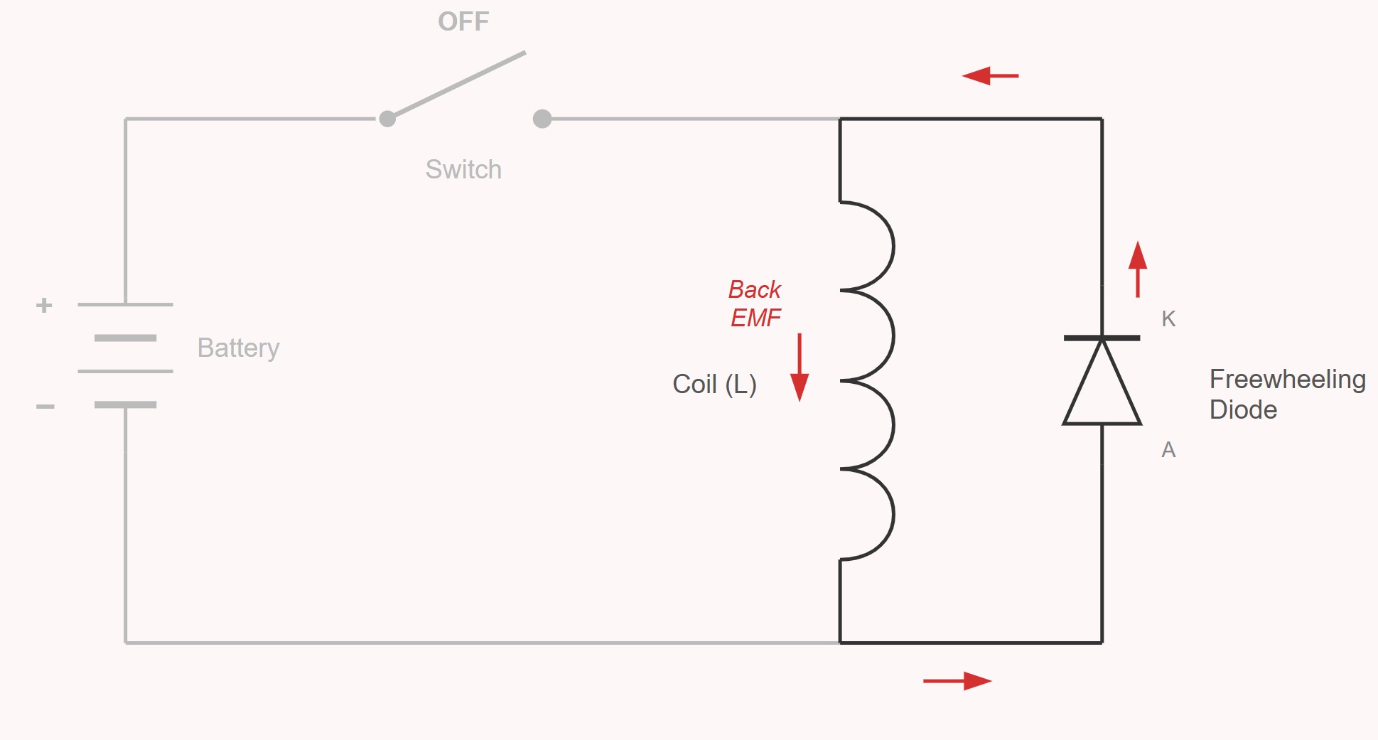 Open Circuit
Then, the current flows through the free-wheeling diode. The current is dissipated itself flowing again into the coil. This behavior makes the magnetic field keep braking the dyno during a few milliseconds as we will see later.
Back to the schematic, next to it is the Free-Wheeling diode which dissipates the stored energy from the coil as previously discussed. Finally there is a protection varistor placed just before the connectors that lead to the eddy current brake.
Additionally the board features several status LEDs to indicate that all necessary voltages are present, the gate driver for the IGBT, and two specific sensors: a voltage divider to monitor the voltage being supplied to the brake and a Hall effect sensor to measure the actual current flow. I will go into more detail on these sensors in a later section.
With the schematic finished it was time to move on to the PCB routing and begin the manufacturing process.
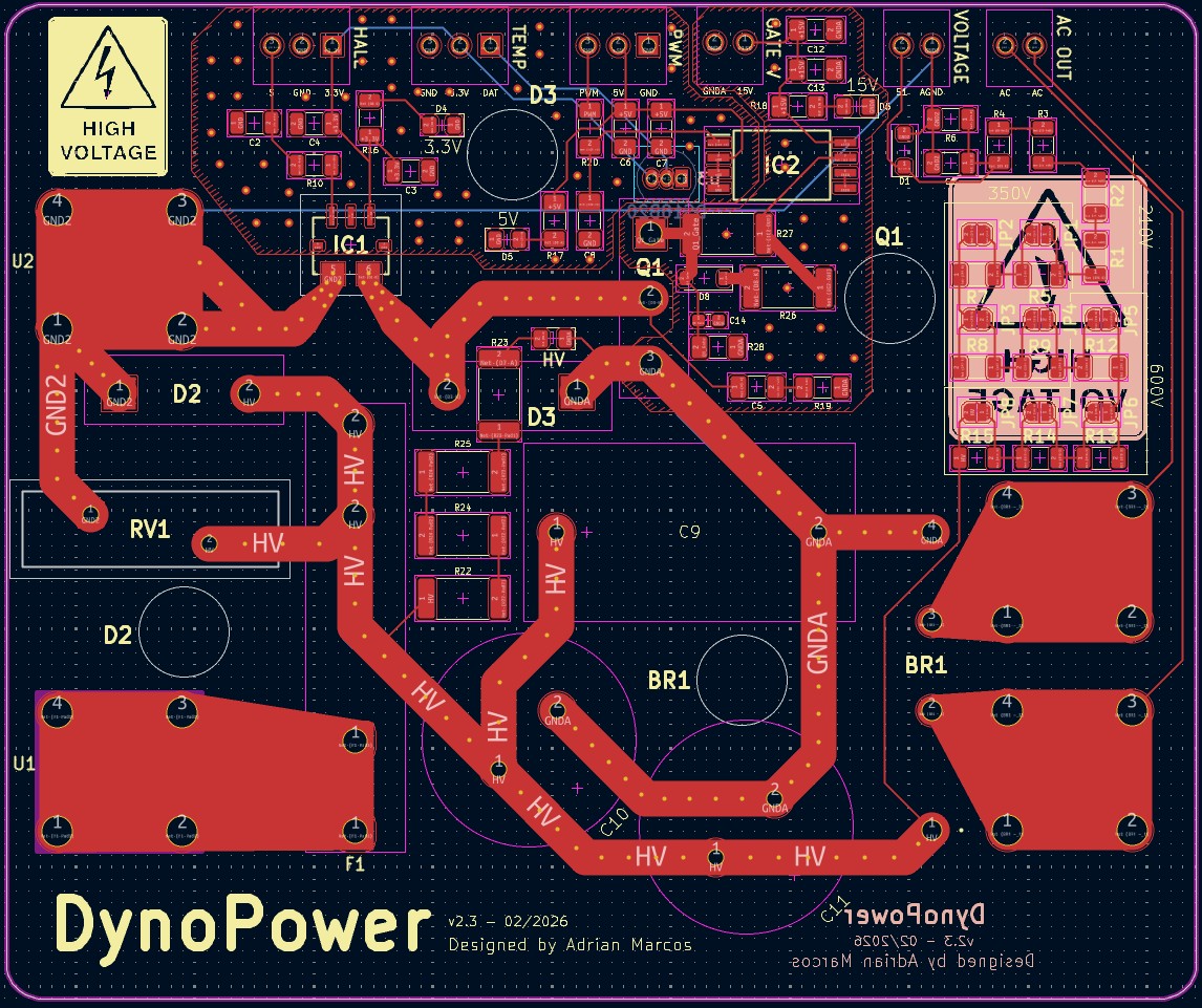 DynoPower V2 Routing
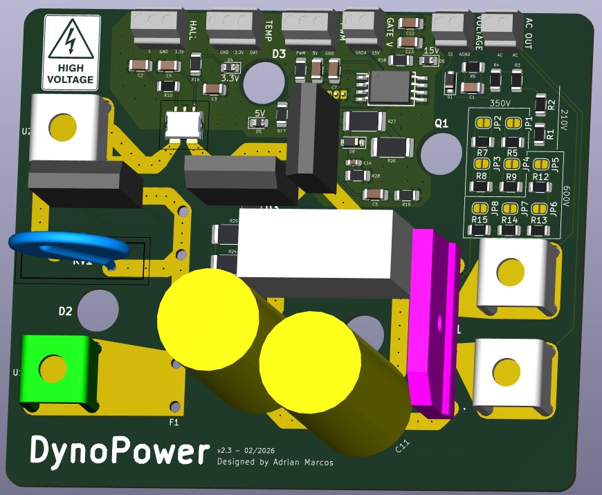 DynoPower V2 3D Render
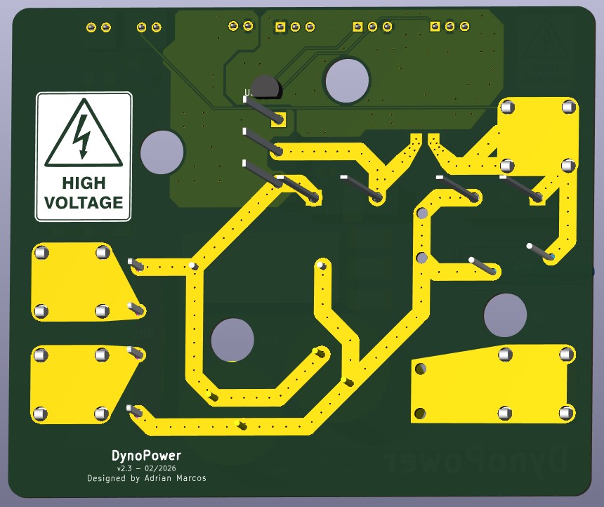 DynoPower V2 Back View
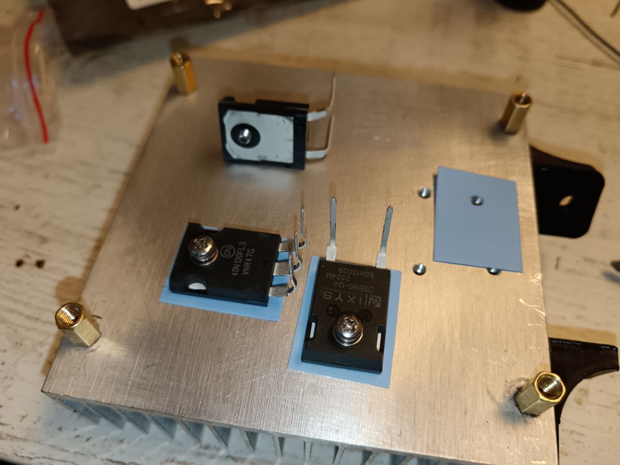 IGBT Thermal Pads
As seen in the previous image, these components feature an exposed metal tab on the back. While this tab is essential for dissipating heat, it is also an active electrical contact, typically the collector. Mounting the IGBTs directly onto an aluminum heatsink would cause a short circuit. To prevent this, I used silicone thermal pads. These are designed to be electrically insulating but thermally conductive, allowing the heat to escape to the heatsink without creating an electrical connection.
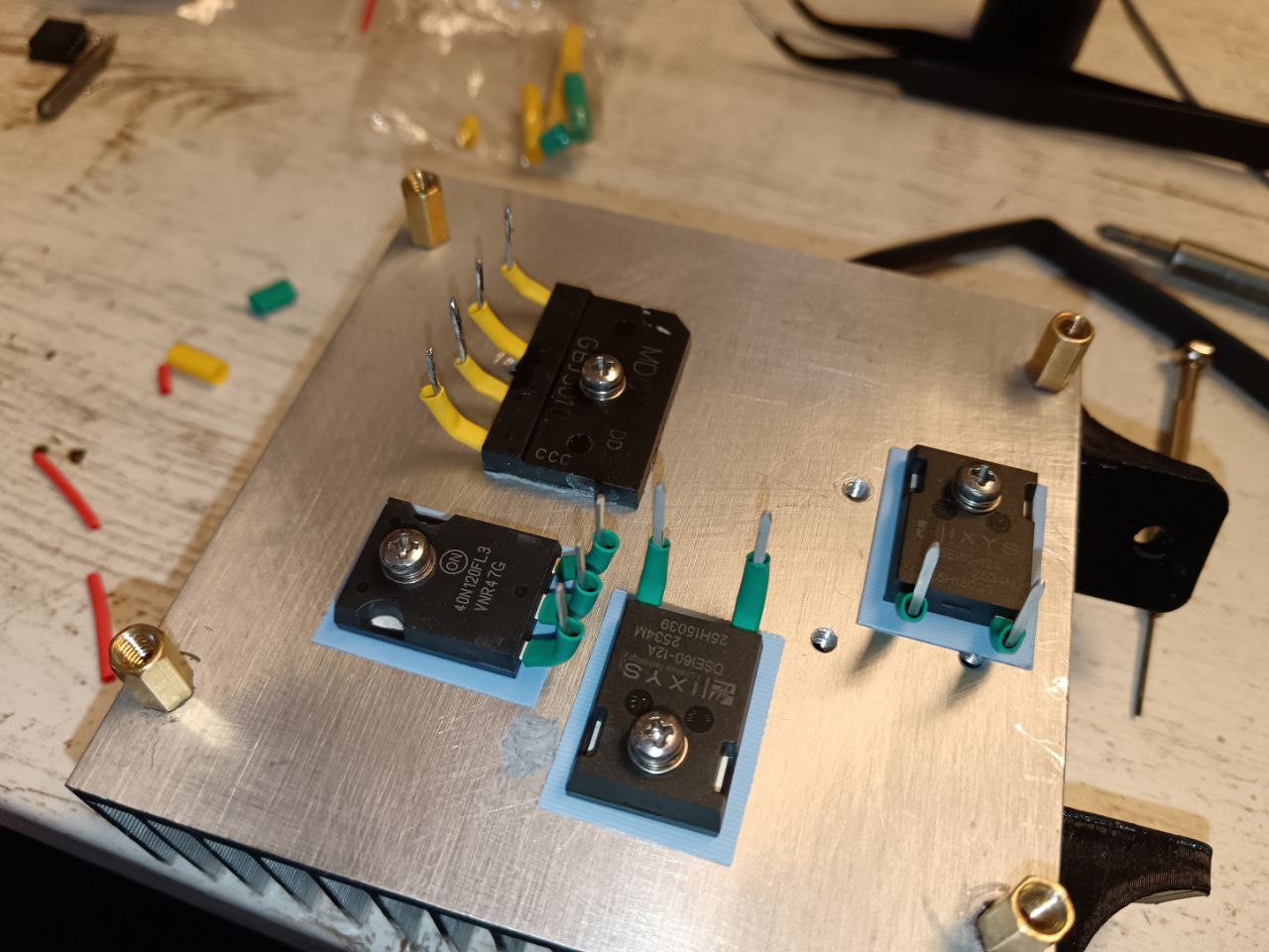 Bridge Rectifier, Diodes and IGBT Mount
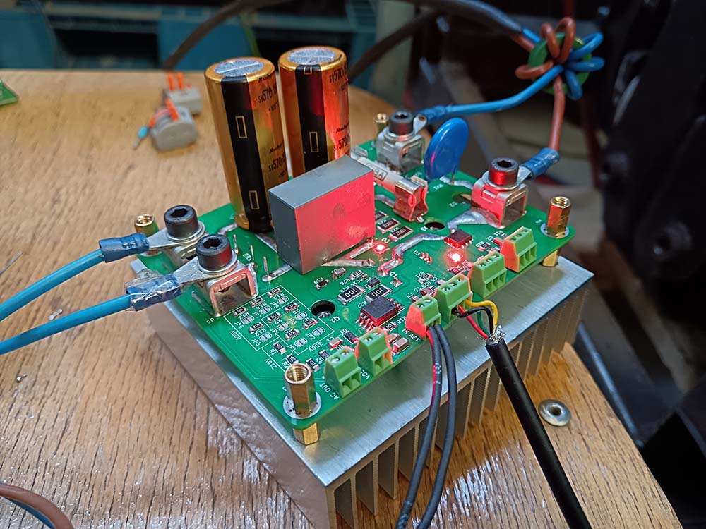 Testing DynoPower V2
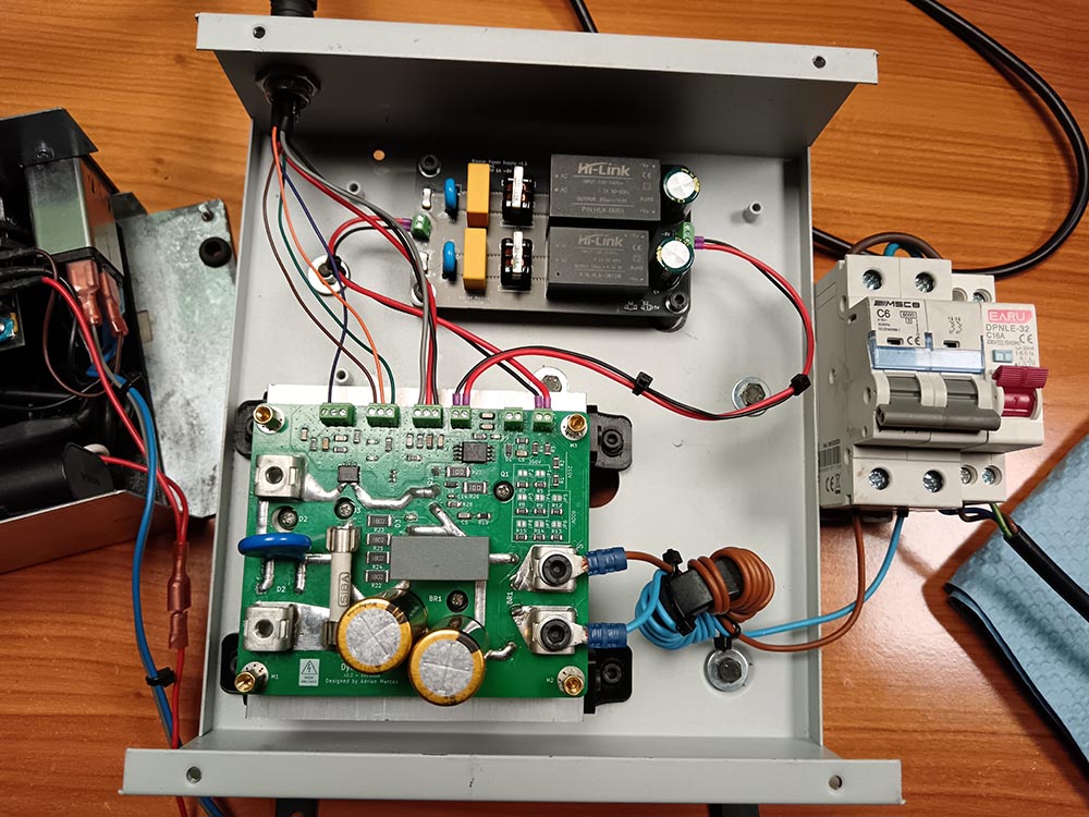 DynoPower V2 with Power Supply
This version worked perfectly and it’s the one that I’m currently using.
To avoid EMI, a choke can be built very easily using a ferrite ring and winding both conductors through it. The goal here is to increase the impedance for high-frequency noise without affecting the DC operation of the system.
The inductance of the choke can be estimated with:
\[L = T^2 \cdot A_L\]Where:
- \(L\) is the inductance
- \(T\) is the number of turns
- \(A_L\) is the ferrite core constant
Both wires must have the same number of turns. Based on Perek’s Help Information6, the required inductance is around 0.5 mH. ${A_L}$ is provided by the ferrite manufacturer.
With that information we can get the following formula:
\[T = \sqrt{\frac{L}{A_L}}\] Ferrite example
Finally, I added a 10 A circuit breaker. This way, if the DynoPower board has any kind of fault or the IGBT becomes stuck in a conducting state, the breaker will trip and prevent potential damage of other components.
Design 3.1 - IGBT with Negative Gate Drive and DESAT (DynoPower v3) (Unfinished)
Unfortunately I could not finish this version successfully. According to the IGBT datasheets, it is highly recommended that when the IGBT is not conducting (the LOW state) the gate should not simply sit at 0V. Instead it is better to apply a negative voltage to the gate. This practice helps prevent accidental conduction caused by external electrical noise or transients. While I have not experienced any issues with the previous version/design yet this was an improvement I wanted to test although I did not manage to get it fully operational.
The first thing I needed was a dedicated power supply for the IGBT gate driver. This supply would need to provide a dual output of +15V and -5V.
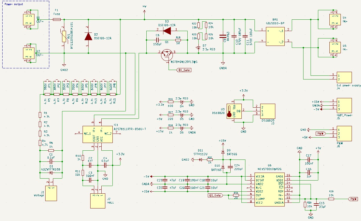 DynoPower v3 Schematic
Bipolar Power Supply
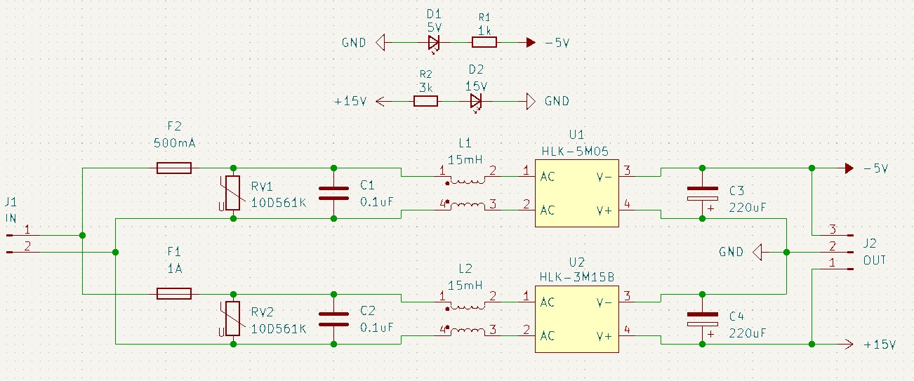 Bipolar Power Supply Schematic
As shown in the schematic I used two AC-DC converters to achieve this function. Since both converters are isolated I could connect their outputs in a specific way to generate a negative voltage reference.
The circuit consists of the following main components:
- HLK-5M05: An AC-DC module that transforms 230VAC to 5VDC.
- HLK-3M15B: An AC-DC module that transforms 230VAC to 15VDC.
Both sub-circuits include these protection and filtering elements:
- Input fuses for overcurrent protection.
- Input varistors to protect against voltage spikes.
- 0.1uF capacitors to filter out high-frequency noise.
- 15mH inductors to clean up the input signal.
On the output side both modules use a 220uF capacitor to stabilize and properly smooth the DC signal. To obtain the -5V rail I connected the GND of the 15V supply to the +5V output of the 5V supply. This creates a center tap that we can use as a common ground reference. Relative to this new GND the output of the 5V module becomes a negative -5V potential as seen in the diagram and the +15V keeps the same value.
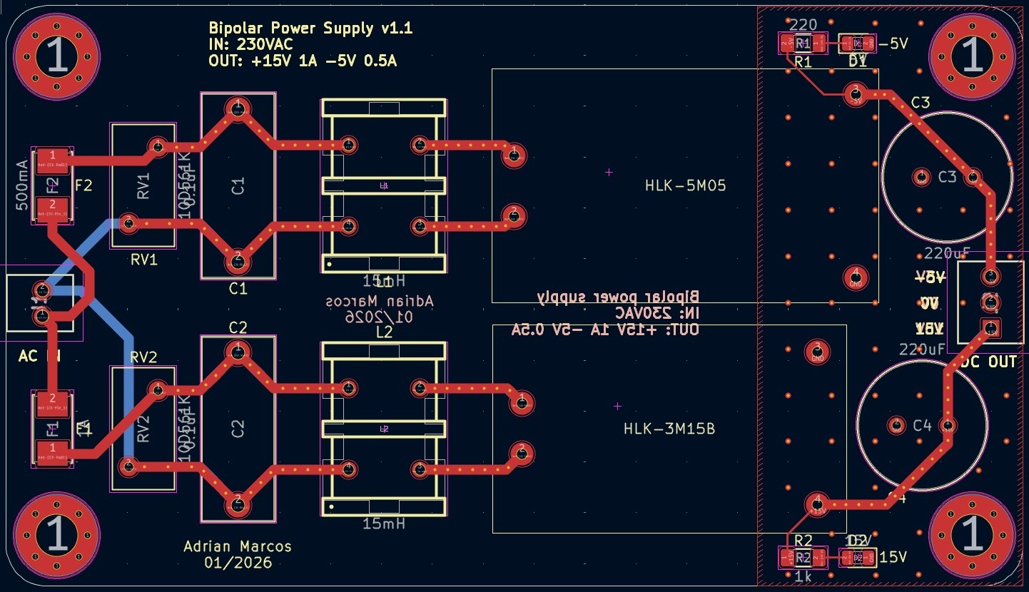 Bipolar Power Supply Routing
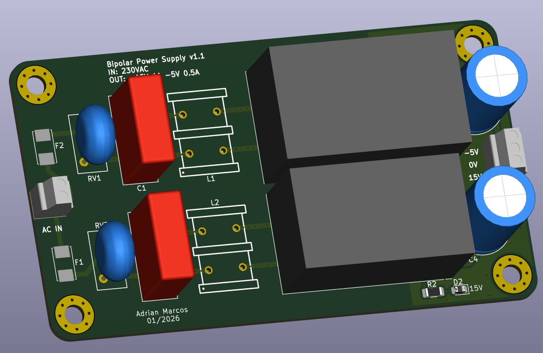 Bipolar Power Supply 3D Render
After completing the PCB design and fabrication this was the final result:
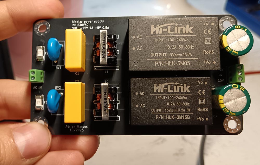 Bipolar Power Supply
This board worked as expected.
Design 4 - IGBT with Fast Discharge Capacitor (Unfinished)
As we saw in the previous designs, I included a free-wheeling diode in anti-parallel with the eddy current brake coils. This diode is used to allow the coil to discharge itself when we stop injecting voltage. When the voltage supply is cut, a reverse polarity voltage is produced and the magnetic field persists for a few milliseconds, depending on the inductance and the current flowing through the coil. We need to discharge that current to stop generating the magnetic field, and that is what the diode is for.
DynoPower V2 Schematic
However, this has a drawback: it slows down the response of the eddy current brake. If the control system decides to stop the current because the brake is applying too much force, the brake will continue braking for a few milliseconds while the energy dissipates, creating a lag. As can be seen in the following graphs, the current actually takes longer to discharge than it does to charge.
On a large dynamometer with a lot of inertia, this is not a significant problem, but on a motor dyno with low inertia, these small delays become noticeable.
This is the standard schematic for discharging through a free-wheeling diode. In this setup, the energy is simply dissipated as heat through the internal resistance of the coils and the diode.
Closed Circuit
Open Circuit
I researched various commercial products that claimed to use a large capacitor for a much faster discharge method. After a lot of thought and many simulations, I designed a circuit that seemed to achieve the behavior I wanted:
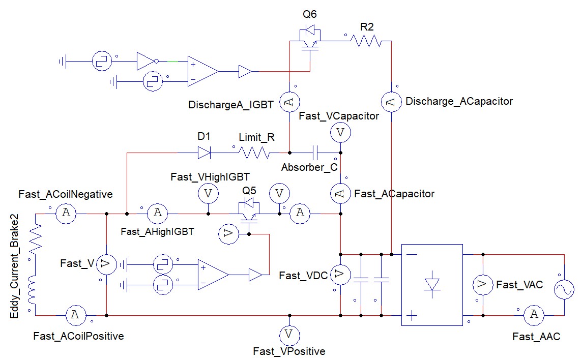 Fast Discharge Schematic
By simulating the system, I obtained the following current graphs:
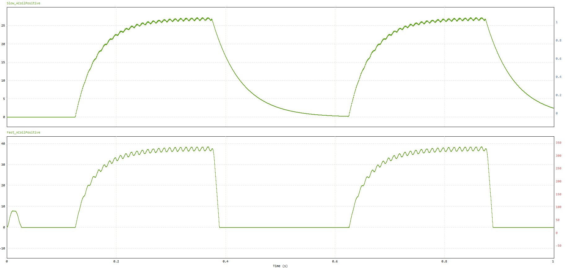 Slow and Fast Discharge Comparison
As we can observe, the brake current discharges much faster in the second graph compared to the standard free-wheeling method. Let’s analyze this schematic in detail:
The initial stage (bottom right) is the same as in previous models. We have the 230VAC input, a bridge rectifier, and capacitors to convert the current to DC. Following this, we find the coil, but unlike the previous case, there is no anti-parallel diode. The circuit then continues to the main IGBT Q5 which cuts the negative side to return to the rectifier.
The difference lies in the parallel branch next to the IGBT. We have a protection diode D1 that limits the return current through that specific path. Following that is a resistor Limit_R used to control the speed at which the absorber capacitor Absorber_C charges. This is necessary because capacitors have very low internal resistance. Without this resistor, the charging process would create a massive current spike that could easily burn out the IGBT Q6.
We have to find a balance for this resistor value: it must be high enough to protect the IGBT but low enough to allow the capacitor to absorb the coil’s energy in the desired time frame.
In parallel with the absorber capacitor, we have the second IGBT Q6. This IGBT conducts when we want to discharge the stored energy from the capacitor. Next to it, resistor R2 acts as another limiter for the capacitor discharge phase.
There are two main things to keep in mind with this design:
- IGBT Gate Management: This requires a microcontroller or a complex logic system capable of controlling both IGBTs simultaneously. Ideally, there should be a small dead-time delay between them.
Let’s analyze the different states in this design. The first state, energizing the coil:
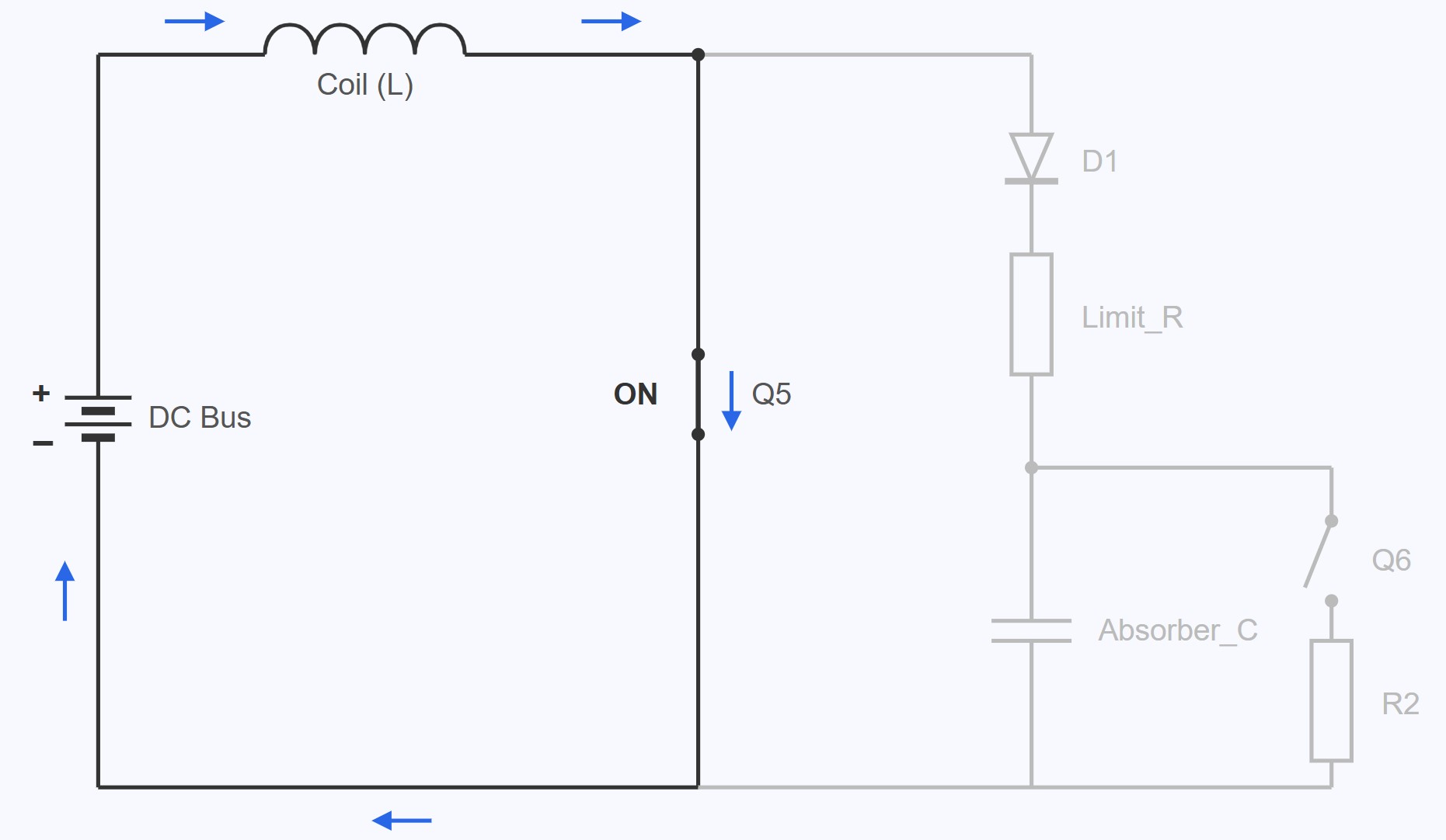 State 1: Energizing the Coil
In this state we can see that the IGBT Q5 is closed so the coil is energized. This is the normal braking state. Let’s move to the next state, the energy absorption by the capacitor:
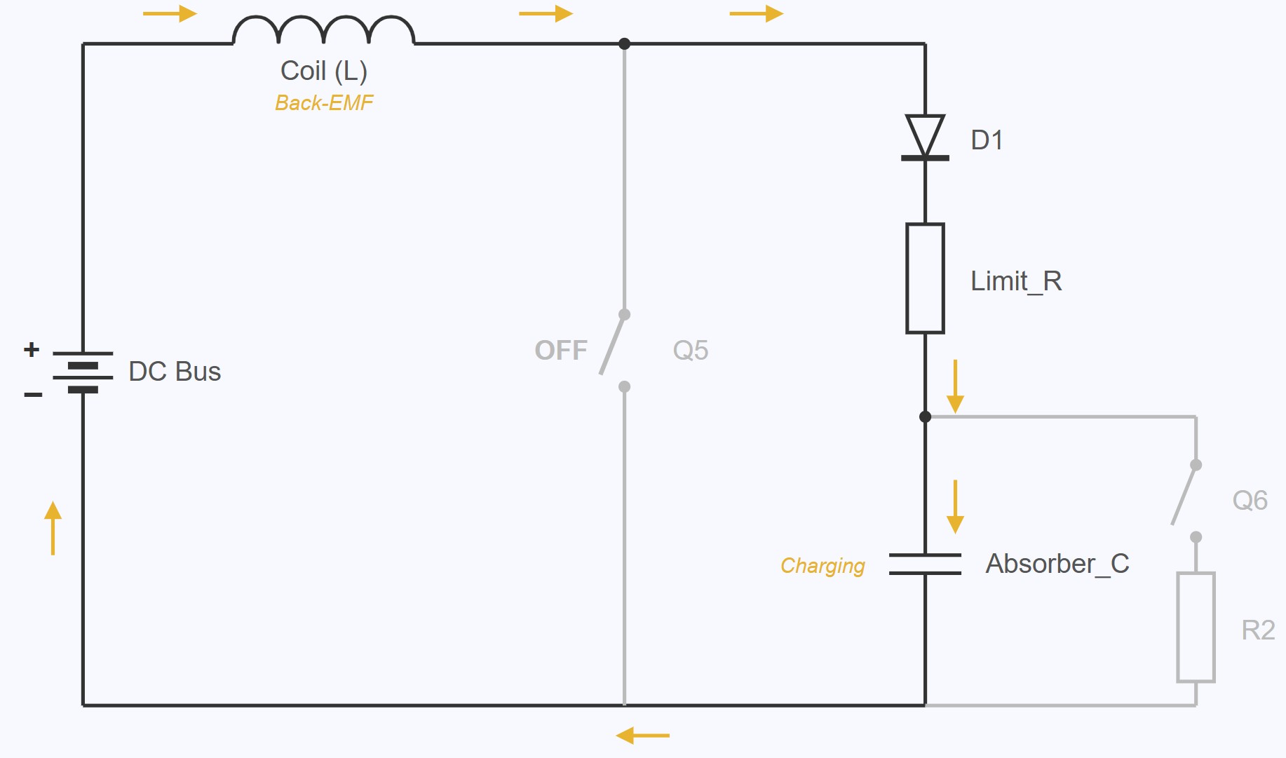 State 2: Capacitor’s Energy Absorption
In this state the IGBT Q5 is turned off. The coil’s back-EMF goes through the D1 and Limit_R and charges the capacitor Absorber_C. This makes the coil to discharge fast and charge the capacitor. We can see that the IGBT Q6 is opened in this state.
Finally, with a small delay after the capacitor Absorber_C has been charged, the IGBT Q6 is closed:
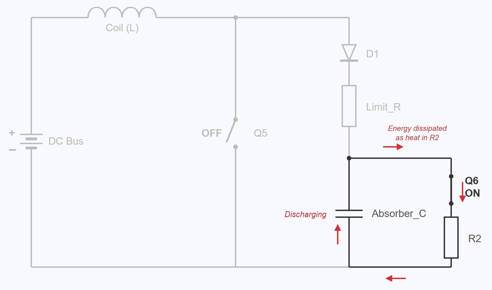 State 3: Capacitor Discharge
When IGBT Q6 is closed, the energy stored in the capacitor Absorber_C is dissipated in R2 as heat.
With this system, the coil is quickly discharged so the magnetic field is removed faster making it a faster torque removal too.
- Capacitor Rating: When the main IGBT
Q5cuts the voltage, the back-EMF produced by the coil can reach values near 1200V. Therefore, the capacitor and the auxiliary IGBT must be rated to handle these high voltages. We also need a relatively large capacitance to handle the energy from the coils.
To determine the required capacitance for the system, we must account for the total magnetic energy ($E_{mag}$) stored in the coils at the moment the IGBT cuts the current. This energy is calculated as:
\[E_{mag} = \frac{1}{2} L I^{2}\]Where:
- $L$ is the inductance of the coils (in Henries).
- $I$ is the peak current flowing through the circuit (in Amperes).
In the following image, we can compare the currents again. The first graph shows the slow discharge and the second shows the fast discharge. The red line represents the voltage applied to the coil, and the green line in the bottom graph shows the IGBT gate signal.
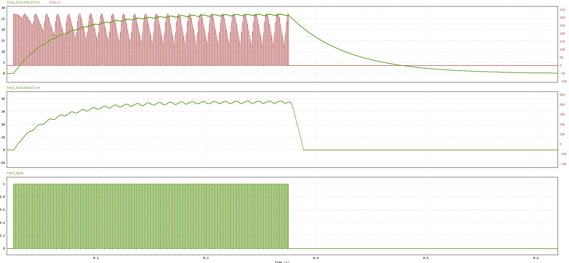 Slow and Fast Current Discharge Comparison with Gate and Voltage Signals
I would have loved to finish this part and verify the real-world differences compared to the free-wheeling diode method, but for personal reasons, I was unable to continue the project.
Design 5 - IGBT with Current Control and Fast Discharge Capacitor (Incomplete)
As I have indicated previously, I was unable to finalize and physically test the results of the previous circuit. Even so, if we wanted to improve the system further (I am not an expert in this area) I believe we could implement the following:
Instead of using a single PID that reads the speed/torque and calculates the current (with the PWM) to be sent to the brake based on that, it would be ideal to have several encapsulated loops. This would mean:
- Current Loop (Inner Loop): We would have a PI loop using a dedicated chip. In this case, this loop would only be responsible for managing the current administered to the brake. To do this, it would handle the IGBT gate and receive feedback on the real current administered to the brake via a current sensor.
- Torque Loop (Middle Loop): Over that PI loop, we could implement a torque loop. In this case, it would use the load cell to read the torque feedback and act on the input of the previous PI loop, telling it what current the system should send to the brake.
- Speed Loop (Outer Loop): Finally, there should be a speed PID loop. This loop would work on the torque loop and would be responsible for adjusting the speed with the reading of the same through the encoder. The same would apply to acceleration.
Below we can see an example of the currently implemented system and what I consider should be the ideal approach for these systems, although I repeat that I am not sure about it, if anyone has any contribution or feedback, it is welcome.
Currently implemented Speed PID
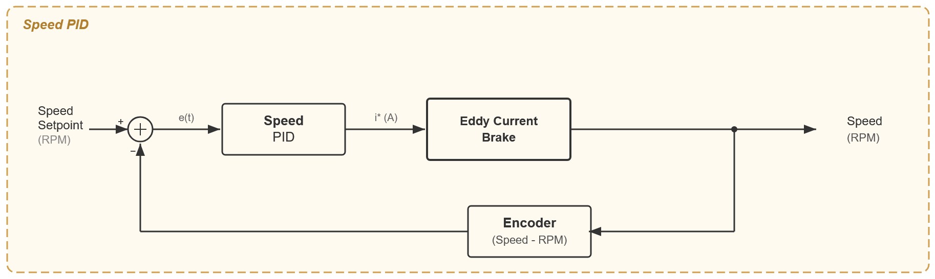 Speed PID
Currently implemented Torque PID
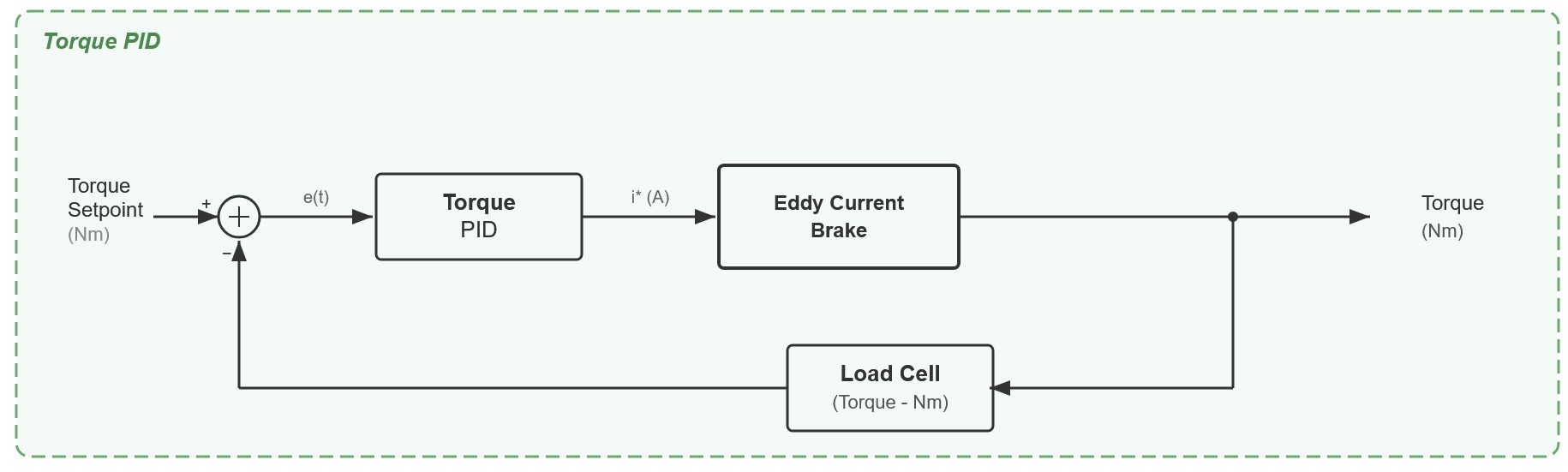 Torque PID
What I think is the best option to implement
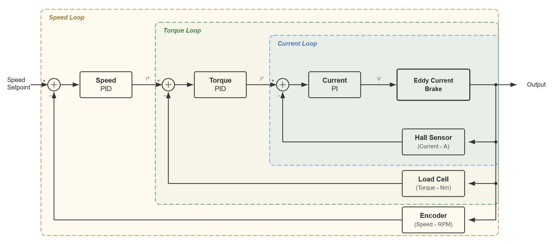 Nested PIDs
Other Sensors
Let’s analyze the other sensors and features implemented in the DynoPower board.
Voltage Divider
Unused in current firmware
My initial idea was to analyze the voltage delivered to the eddy current brake to perform more precise braking calculations, but I ultimately decided to set this option aside. Nevertheless, the DynoPower board includes a voltage divider to measure the voltage being injected into the brake.
As we will see later, to measure the voltage from the logic board (DynoLogic), I use an isolated ADC with a maximum input of 1.8V. This means I need to step down the voltage from a 325V peak to 1.8V. Furthermore, as previously mentioned, the back-EMF from the eddy current brake coils can generate voltage spikes even higher than that. The PCB is equipped with a voltage divider capable of handling up to 600V. It is worth noting that I have not tested this connection to date, so if someone replicates the project and does not plan to use it, I recommend leaving it disconnected.
To mitigate potential interference, the strategy was for this PCB to step the voltage down to a safer intermediate level before passing it to the DynoLogic board, which would then handle the final reduction to 1.8V. I am not entirely certain if this multi-stage reduction has a significant impact on signal integrity, but the goal was to avoid transmitting a sensitive 1.8V signal across different boards.
Hall Current Sensor
 ACS781LLRTR-050U-T
Just like in the previous case, I was initially interested in measuring the current flowing through the coil, both to understand the power consumption of the eddy current brake and to implement some type of safety control.
For this purpose, I selected the ACS781LLRTR-050U-T sensor. This sensor operates based on the Hall effect and supports a maximum of 50A, which is more than enough for my application.
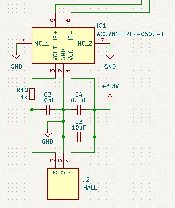 ACS781LLRTR-050U-T Schematic
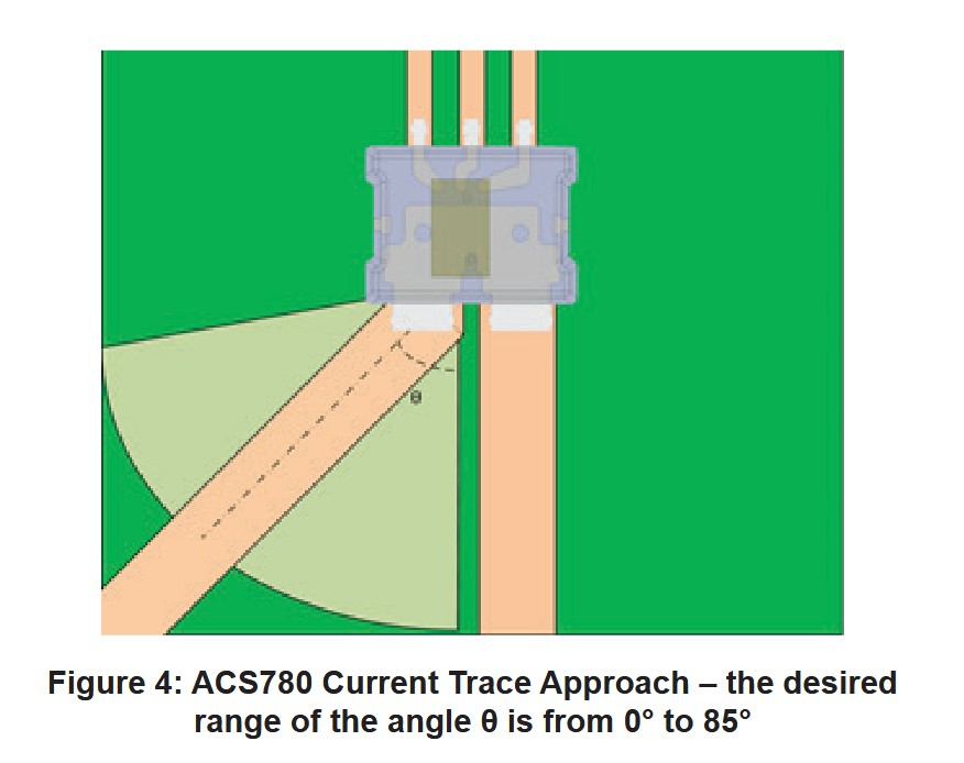 ACS781LLRTR-050U-T Datasheet
One of the main advantages of using a Hall effect sensor is that it provides galvanic isolation between the high-power circuit and the logic side. This is essential for protecting the microcontroller from the high voltages used to drive the brake. The sensor outputs an analog voltage proportional to the current detected in the primary conductor. This specific sensor has unidirectional current detection (positive) and it can sample a maximum of 50A with a sensitivity of 39.6 mV/A.
As seen in the schematic, this chip requires decoupling capacitors and resistors to suppress high-frequency (HF) noise. Additionally, careful attention must be paid to trace routing and PCB layout. These guidelines are clearly explained in the datasheet.
DS18B20 (Temperature Sensor)
To monitor the temperature of the DynoPower board, I used a DS18B20 sensor. Although in my application I am unlikely to ever overheat the heatsink because I work with very low currents (10A peak, but my actual use will likely be around 3A), I decided to design the board to support larger brakes. For this, I use a One-Wire type sensor to collect the temperature from the heatsink.
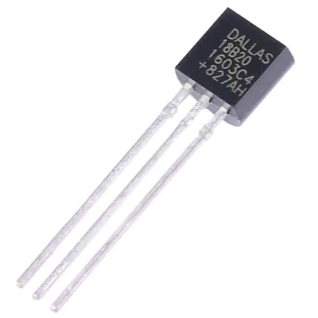 DS18B20
This sensor works with the One-Wire protocol. This means we only need 3 pins to connect to the microcontroller:
- VDD: Power Supply Voltage (accepts 3.0V to 5.5V).
- GND: Ground signal.
- DQ: Data In/Out.
With these 3 pins, it is enough to send the temperature data to the microcontroller. The schematic, as you can see, is remarkably simple:
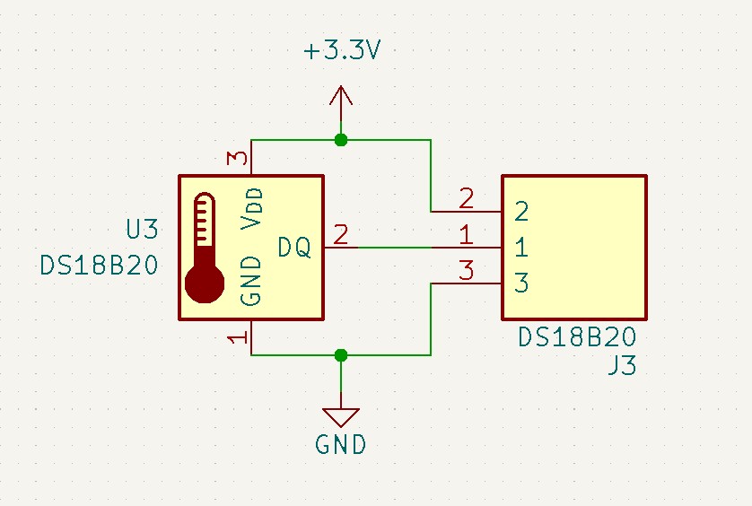 DS18B20
Onboard LEDs
This feature was not included in the early versions, as these are ideas that evolve over time. To ensure the entire system functions correctly, I introduced three low-voltage LEDs: one to verify the 3.3V supply, another for 5V, and a third for the 15V that powers the IGBT driver.
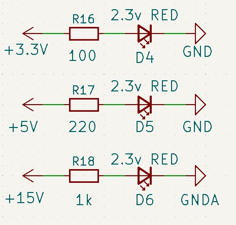 DynoPower LV LEDs
To calculate the appropriate resistor values, we use Ohm’s Law:
\[\begin{aligned} R = \frac{V_{in} - V_f}{I_f} \end{aligned}\]While standard red LEDs can typically handle a maximum continuous forward current ($I_f$) of 20mA, running them at around 10 to 12mA provides more than enough brightness for a panel indicator while improving efficiency and component lifespan. Given an LED forward voltage ($V_f$) of 2.3V, we can calculate the exact values used in the schematic:
3.3V Line
\[\begin{aligned} R = \frac{3.3V - 2.3V}{0.010A} = 100\Omega (R16) \end{aligned}\]5V Line
\[\begin{aligned} R = \frac{5.0V - 2.3V}{0.0121A} \approx 220\Omega (R17) \end{aligned}\]15V Line
\[\begin{aligned} R = \frac{15.0V - 2.3V}{0.0127A} = 1k\Omega (R18) \end{aligned}\]Using these standard resistor values guarantees a safe operating current for the LEDs across all low-voltage rails without pushing them to their absolute limits.
From my perspective, the most interesting and important LED is the high-voltage indicator:
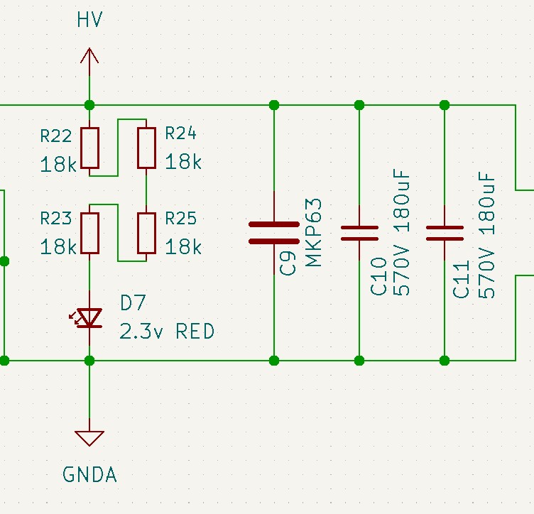 DynoPower HV LED
In this case, the LED indicates that high voltage is present in the system. Beyond serving as a safety warning, it solves a specific problem I encountered: the board’s capacitors could hold a significant charge for days after being unplugged. With this LED circuit, the capacitors self-discharge through the series resistors and the LED shortly after the system is turned off.
Operating at such high voltages requires careful consideration of both power dissipation and component voltage ratings. To determine the resistor setup for the HV line (assuming a peak of roughly 300V), I intentionally targeted a much lower forward current to keep temperatures manageable while still maintaining visibility.
The circuit uses four $18k\Omega$ resistors in series, resulting in a total resistance of $72k\Omega$. The current flowing through the LED is:
\[I = \frac{300V - 2.3V}{72000\Omega} \approx 4.1mA\]Even at 4.1mA, the LED is visibly bright enough to serve as a reliable warning. More importantly, we must look at the power dissipated as heat. The total power dissipated by the resistor chain is:
\[P_{total} = (300V - 2.3V) \times 0.0041A \approx 1.22W\]By splitting this load across four resistors in series, each one only dissipates roughly $0.30W$ ($1.22W / 4$). Furthermore, standard SMD resistors often have a maximum working voltage rating (e.g., 150V or 200V). Distributing the nearly 300V drop across four components ensures that each resistor only sees about $75V$, keeping them safely within their operating margins and preventing arcing.
Finally, this $72k\Omega$ resistance forms an RC circuit with the two $180\mu F$ bulk capacitors ($360\mu F$ total). With a time constant ($\tau$) of roughly $26$ seconds ($72000\Omega \times 0.000360F$), the capacitors will safely self-discharge to near zero volts in just a couple of minutes after the system is powered down.
With the DynoPower stage finished, let’s dive into the DynoLogic board.
DynoLogic
General Requirements
Once the power stage was finished, it was time to start with the system’s logic stage. This stage is responsible for the real-time control of the dynamometer and managing safety protocols to prevent mechanical and electrical failures. The system must be capable of measuring the speed of the eddy current brake, the torque generated (via the load cell), as well as temperatures and other auxiliary sensors. Based on this data, it must then send the appropriate control commands to the DynoPower board.
To ensure high-fidelity measurements and a fast response time, I established the following requirements for this board:
- Real-Time Processing: The control loops (especially the PID) must run at a consistent, high frequency to ensure the brake responds immediately to demand changes.
- Galvanic Isolation: Since the DynoPower board handles high voltages (up to 325V peak), the logic board must be isolated to protect the microcontroller and any connected user devices (like a laptop or DynoServer board).
- Sensor Integration: Native support for high-precision ADCs for the load cell, high-speed interrupt pins for the encoder, and One-Wire/I2C buses for temperature monitoring.
- Reliability: The environment near an engine is electrically noisy. The board needs proper decoupling and shielding to prevent electromagnetic interference (EMI) from causing crashes or false readings.
With these requirements defined, I began selecting the brain of the system and designing the PCB layout.
Microcontroller
Initially, I planned to use an Atmel SAM3X8E as the brain of the system. The main reason was practical: I had several modules in stock at home and wanted to put them in use. These modules were the “Due Core” shown below:
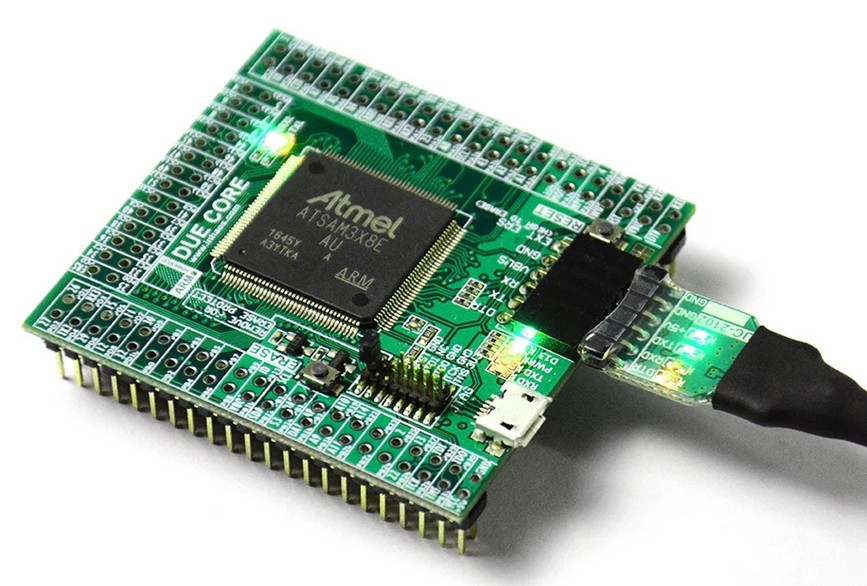 Due Core Board
The specifications for this microcontroller were as follows:
| Feature | Specification |
|---|---|
| Processor | ARM Cortex-M3 (Atmel SAM3X8E) at 84 MHz |
| Flash Memory | 512 KB Flash |
| RAM (SRAM) | 96 KB SRAM (divided into two banks: 64 KB and 32 KB) |
| USB | 1x Native USB port, 1x Programming USB port |
| Digital I/O Pins | 54 digital input pins (not 5 V compatible) |
| Analog Input Pins | 12 analog input pins (0 to 3.3 V max) |
| PWM Pins | 12 PWM Pins with 8 bits resolution |
| Communication Ports | 4x UART, 2x I2C, 1x SPI |
| CAN Bus | 2x CAN controllers (requires external transceiver) |
| DMA | Built-in DMA controller |
| RTC | Built-in Real-Time Clock |
The first version I built worked, but it suffered from compatibility issues with the I2C protocol when reading temperatures. I went through several board iterations trying to refine the design, but after accidentally burning out one of the modules, I decided to switch to a superior microcontroller. It wasn’t because I needed more power, it was because of the price. The SAM3X8E was becoming more expensive and harder to find than the Teensy 4.1, which offered significantly better features for a lower price.
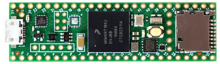 Teensy 4.1
The specifications for the Teensy 4.1 are:
| Feature | Specification |
|---|---|
| Processor | ARM Cortex-M7 at 600 MHz |
| Flash Memory | 7936 KB Flash |
| RAM (SRAM) | 1024 KB RAM (512K tightly coupled) |
| USB | 1x USB device (480 Mbit/sec), 1x USB host (480 Mbit/sec) |
| Digital I/O Pins | 55 digital input/output pins |
| Analog Input Pins | 18 analog input pins |
| PWM Pins | 35 PWM output pins |
| Communication Ports | 8x Serial (UART), 3x I2C, 3x SPI |
| CAN Bus | 3x CAN Bus (1 with CAN FD) |
| DMA | 32 general purpose DMA channels |
| RTC | RTC for date/time |
With the 600 MHz clock speed of the Teensy 4.1, the real-time control loops have a massive amount of overhead, ensuring that calculations never lag. Now that the brain of the system is chosen, let’s dive into the specific sensors used.
Encoder
The first thing we need to measure is the rotational speed of the eddy current brake. And trust me, it’s harder than what you think. This speed is related to the gear ratio to the motor’s RPM since they are mechanically linked by a chain. There are several ways to capture this data:
- Resolver: It uses analog sine/cosine waves to measure position and speed.
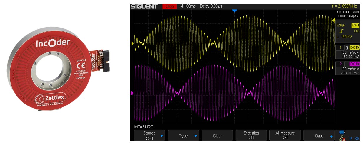 Resolver
- Encoder: The most common digital solution. It uses a disc (optical or magnetic) to generate pulses.
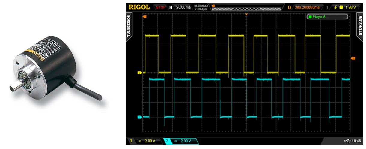 AB Encoder
- Hall Effect Sensor: Uses magnets mounted on the shaft. It is very cheap and immune to dust/oil, but usually offers much lower resolution (PPR) than an optical encoder.
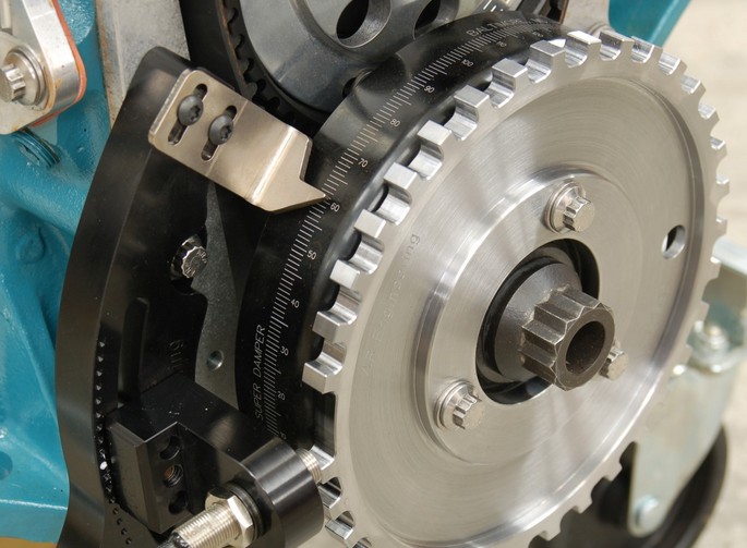 Hall Sensor
Absolute vs. Incremental Encoders
It is important to distinguish between these two types. An Absolute Encoder knows its exact angular position at all times, even after a power cycle, thanks to a unique pattern for every degree of rotation. An Incremental Encoder (like the one I used) simply counts pulses relative to a starting point. For a dynamometer where we primarily care about RPM (speed) rather than the exact stop-start position of the shaft, an incremental encoder is the standard and more cost-effective choice.
I decided to go with an AB Phase Incremental Encoder, as seen here:
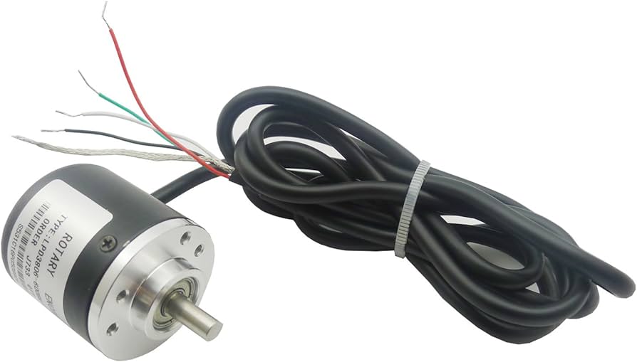 AB Encoder
Encoder Internals
For those curious about the “magic” inside, here is a look at the internal disc:
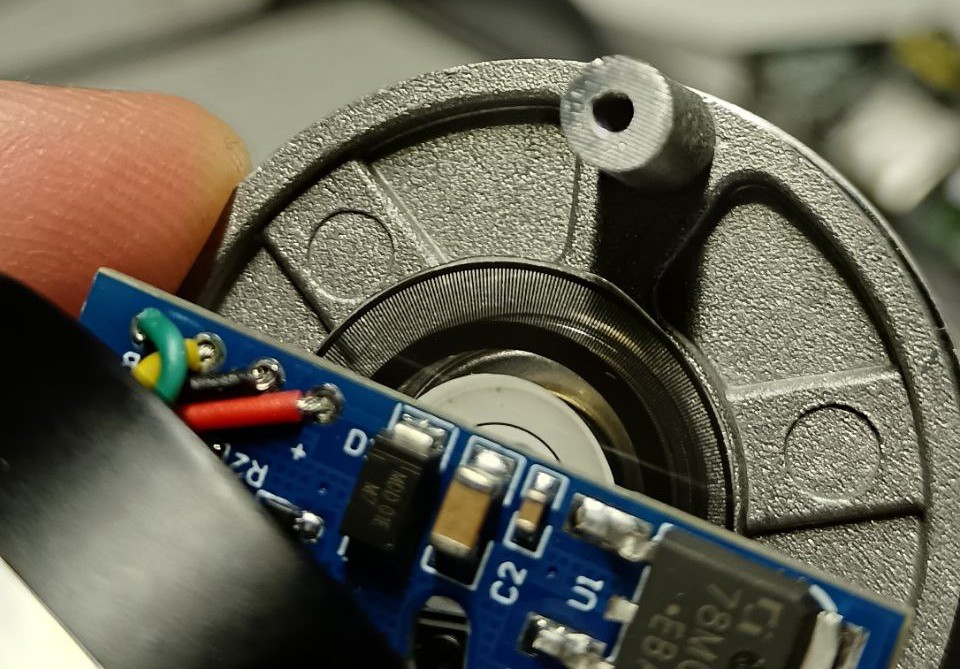 AB Encoder
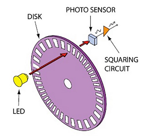 AB Encoder
The operation is fundamentally simple: a LED shines light toward a receiver. As the disc spins, the black lines block the light beam while the transparent gaps allow it to pass. The internal electronics convert these light flickers into a clean square wave signal.
The resolution is measured in PPR (Pulses Per Revolution). Common values are 360, 600, or 1000 PPR. While higher PPR provides better resolution at low speeds, it can overwhelm a slow microcontroller at high RPMs. Fortunately, with the Teensy 4.1 running at 600 MHz, we can handle very high pulse frequencies without breaking a sweat.
Understanding Open Collector Outputs
Many industrial encoders, including the one I used, feature an Open Collector output. If you look at the internal diagram below, you will notice the output is basically the “Collector” of an internal NPN transistor left “open.”
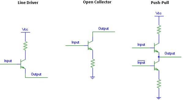 Open Collector Diagram
In this configuration, the encoder does not “push” a high voltage, it only “pulls” the signal to Ground (0V). To read this with a microcontroller, we must use a Pull-up Resistor. This resistor pulls the signal line up to our logic voltage (3.3V or 5V). When the encoder transistor switches on, it shorts the line to ground, creating the “Low” pulse. This is actually a great feature for our project because it allows us to power the encoder at 12V or 24V for better noise immunity while safely interfacing with our 3.3V logic board just by choosing the right pull-up voltage.
Schmitt Trigger
One of the primary challenges with AB encoders is electrical noise. Despite using shielded cables, dyno environments are “dirty” due to high-speed switching transistors (IGBTs) and 3-phase AC motor spinning nearby. After struggling to filter this noise efficiently via software which often introduces unwanted latency, I decided to solve it at the hardware level.
To do this, I implemented a Schmitt Trigger.
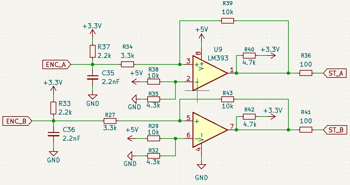 Schmitt Trigger with LM393
As shown in the schematic, by using a dual comparator like the LM393 (one for signal A and one for signal B), we can clean up the encoder signal. Let’s look at the behavior in the following graph:
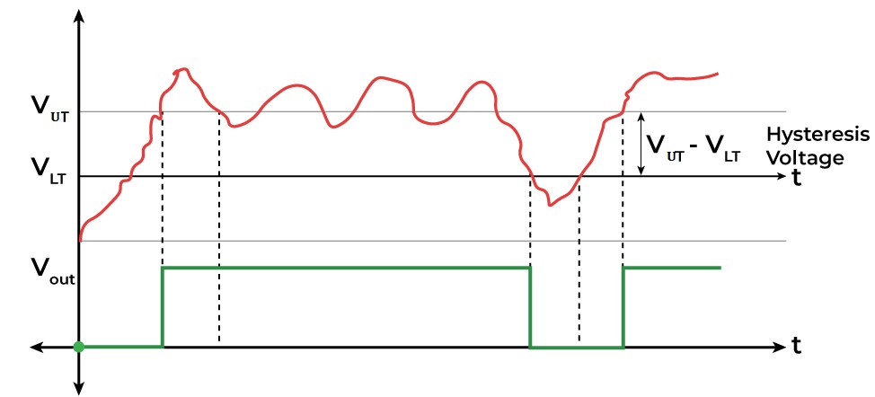 Schmitt Trigger7
By choosing specific resistor values, we set an Upper Threshold Voltage ($V_{UT}$) and a Lower Threshold Voltage ($V_{LT}$).
- The output only switches to HIGH if the input signal rises above $V_{UT}$.
- The output only switches to LOW if the input signal drops below $V_{LT}$.
The area between these two points is known as the hysteresis band.
How it Works
Imagine our encoder signal operates between 0V and 3.3V. Without a Schmitt Trigger, a microcontroller might assume any voltage above 1.65V is HIGH. If the signal is currently LOW (0V) but a burst of EMI creates a noise spike of a bit more than 1.8V, the microcontroller will register a false pulse. This ruins your RPM readings.
With the Schmitt trigger, we can tune the circuit so it does not consider the signal HIGH until it hits 3.0V, and does not consider it LOW again until it drops below 0.8V. If we are at 0V and that same 1.8V noise spike hits, the output stays LOW because it never crossed the 3.0V threshold. This hardware-level filtering ensures the Teensy 4.1 receives a clear signal regardless of the electrical noise happening nearby.
To find the trigger voltages, we first need to determine the reference voltage ($V_{ref}$) applied to the inverting input (pin 2). This is set by the voltage divider formed by R38 (10k) and R35 (4.3k) connected to +5V.
Now we calculate the thresholds for the input signal $V_{in}$ (the voltage at the node where R37, C35, and R34 meet).
Upper Threshold ($V_{TH}$)
This is the voltage required to switch the output from LOW to HIGH. When the output is LOW, the LM393 pulls pin 1 to ground ($0V$).
\[\begin{aligned} R_{in} = 3.3k\Omega (R34) \end{aligned}\] \[\begin{aligned} R_f = 10k\Omega (R39) \end{aligned}\] \[\begin{aligned} V_{TH} = V_{ref} \times \left(1 + \frac{R_{in}}{R_f}\right) \end{aligned}\] \[\begin{aligned} V_{TH} = 1.50V \times \left(1 + \frac{3.3k\Omega}{10k\Omega}\right) = 1.50V \times 1.33 \approx \textbf{2.00V} \end{aligned}\]Lower Threshold ($V_{TL}$)
This is the voltage required to switch the output from HIGH to LOW. When the output is HIGH, the LM393 stops pulling to ground, and the node is pulled up to +3.3V ($V_{pullup}$) via R40 (4.7k). This pull-up resistor becomes part of the feedback network.
Summary:
- Switches HIGH at: 2.00V
- Switches LOW at: 1.10V
- Hysteresis Band: 0.90V
How to Calculate Resistors for a Desired Voltage
Designing this specific open-collector topology backwards (from desired voltages to resistor values) requires a bit of iteration because the pull-up resistor ties the variables together.
Step 1: Lock in your standard parameters
Choose fixed values for your pull-up voltage, your pull-up resistor, and your feedback resistor.
- $V_{pullup} = 3.3V$
- $R_{pullup} = 4.7k\Omega$ or $10k\Omega$
- $R_f = 10k\Omega$ or $100k\Omega$
Step 2: Choose a Reference Voltage ($V_{ref}$)
Your reference voltage must be somewhere between your desired $V_{TL}$ and $V_{TH}$. A good starting guess is slightly below the midpoint of your desired thresholds.
Step 3: Calculate the required Input Resistor ($R_{in}$)
Using your target Upper Threshold ($V_{TH}$), calculate what $R_{in}$ needs to be:
\[R_{in} = R_f \times \left( \frac{V_{TH}}{V_{ref}} - 1 \right)\]Step 4: Verify the Lower Threshold ($V_{TL}$)
Insert the $R_{in}$ you just calculated into the $V_{TL}$ formula to see where your lower threshold lands:
\[V_{TL} = V_{ref} - \left( \frac{V_{pullup} - V_{ref}}{R_f + R_{pullup}} \times R_{in} \right)\]Step 5: Iterate if necessary
- If your calculated $V_{TL}$ is too high, you need to decrease your $V_{ref}$ and recalculate from Step 3.
- If your calculated $V_{TL}$ is too low, you need to increase your $V_{ref}$ and recalculate from Step 3.
Load Cell
One of the most critical requirements of this project is measuring the torque generated by the motor. As previously mentioned, I use a load cell to achieve this.
A load cell is a transducer that converts mechanical force into an electrical signal. This data allows the electronics to calculate the torque produced by the motor by measuring the force exerted at a specific distance (the lever arm). Most load cells use strain gauges arranged in a wheatstone bridge circuit to detect microscopic deformations in the metal body of the sensor.
How Load Cell Works?
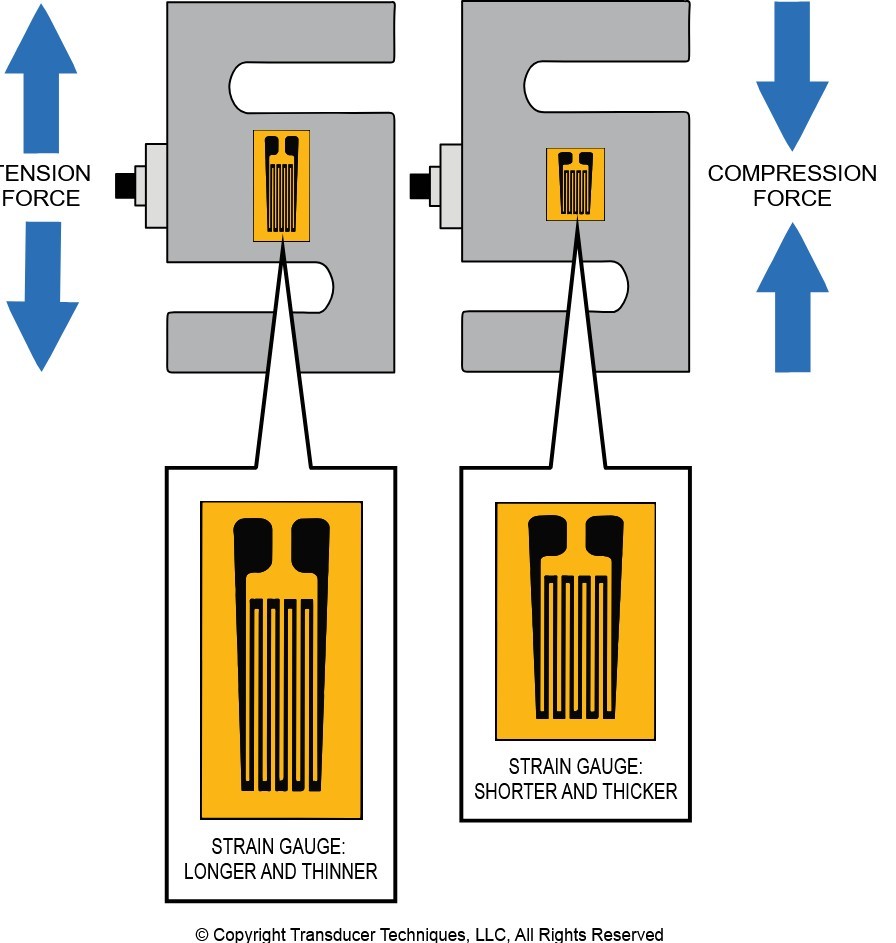 Load Cell Operation
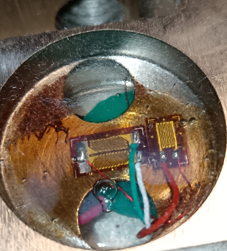 Load Cell Internals
As seen in the images, a load cell is essentially a precision-machined piece of metal, in this case, an S-type cell. At the center of the “S” there is a specific machined area forming a thin internal wall. The thickness of this wall determines the maximum capacity of the load cell.
Strain gauges are bonded to this wall. When a load is applied to the cell, this thin metal section undergoes elastic deformation. While these changes are invisible to the eye, they are enough to change the electrical resistance of the gauges. The microcontroller, usually via an amplifier/ADC like the HX711, detects this variation as a change in voltage, allowing the system to calculate the exact force applied with high precision.
An important characteristic of S-type load cells is that they can measure force in both directions: tension (pull) and compression (push). I designed the dyno with a push system in early stages of the project. Both options are valid but perhaps setting it as pull allows the self-alignment of the forces in the reaction arm and reduces a bit the vibration of the structure applied to the load cell.
Load Cell Amplifier (HX711)
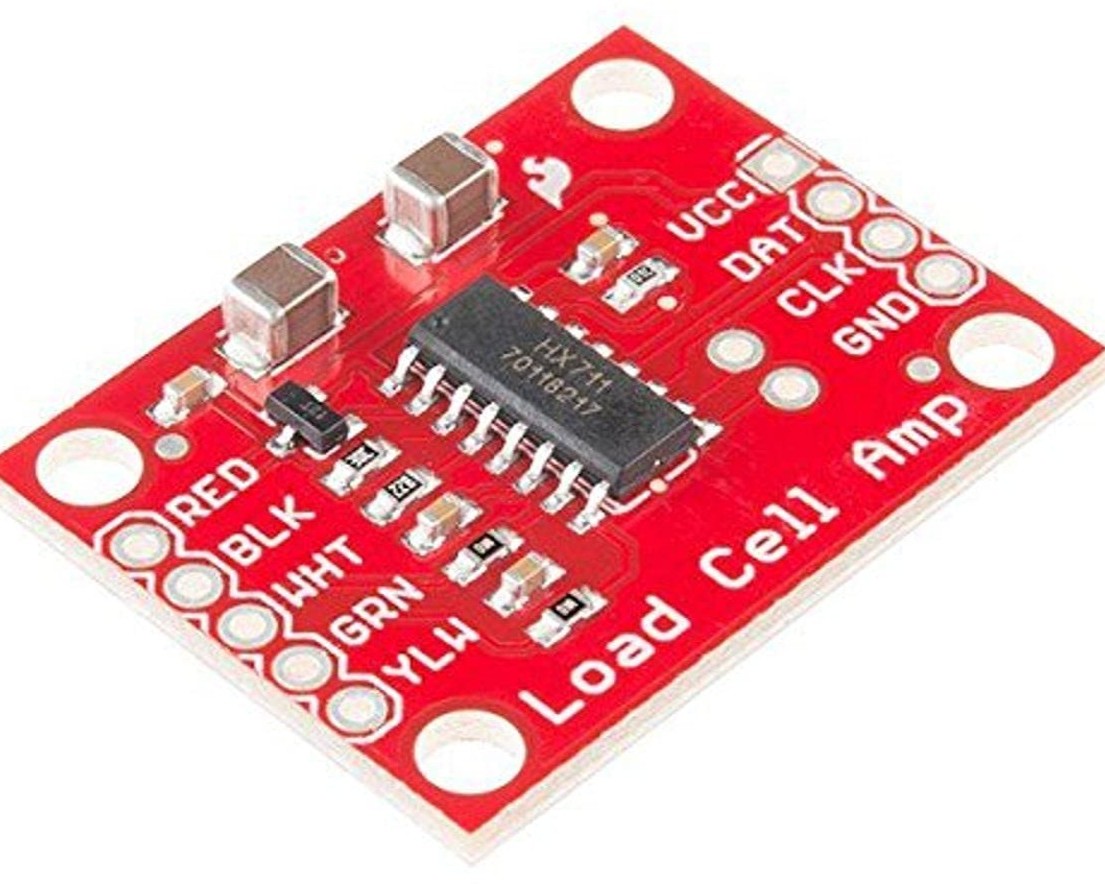 HX711 Board (Front)
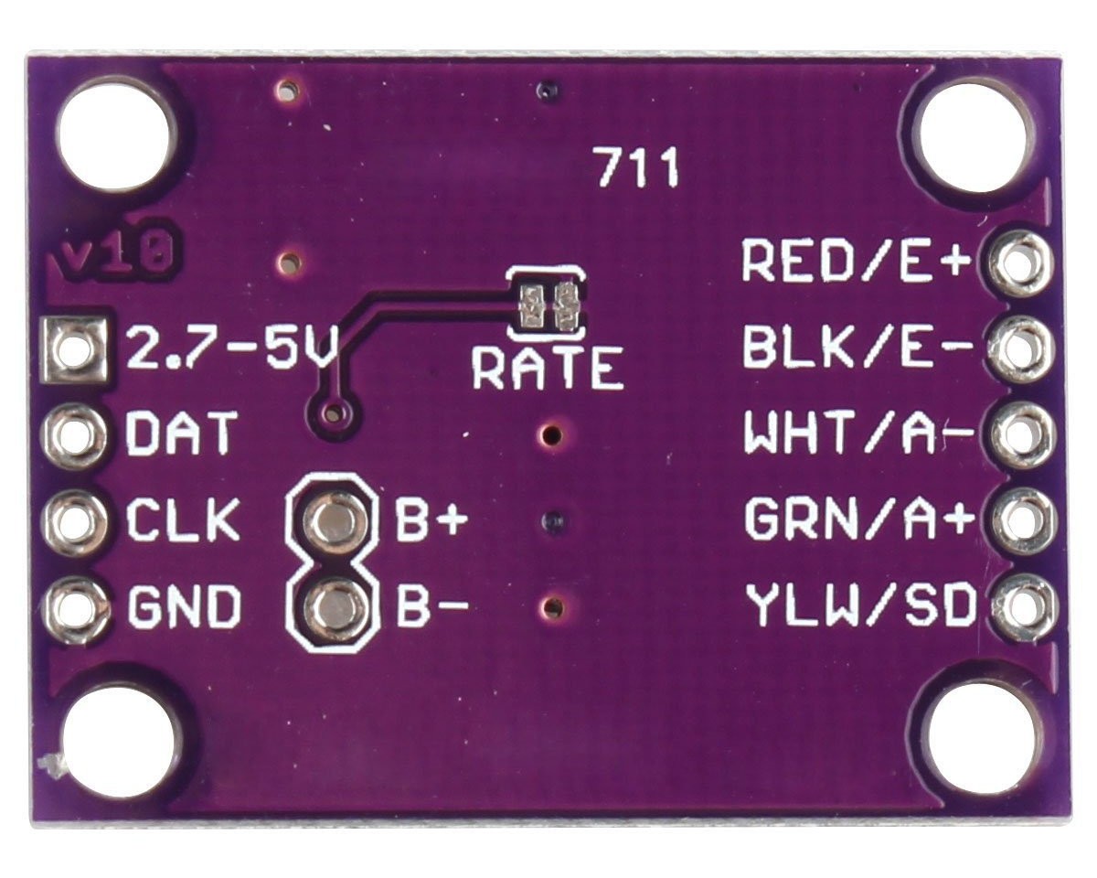 HX711 Board (Back)
Load cells operate using strain gauges arranged in a Wheatstone bridge circuit. When force is applied, the physical deformation slightly changes the resistance of the gauges, outputting a differential voltage. However, this voltage change is microscopic, typically in the range of just a few millivolts (mV) even at maximum load.
If you try to read this signal directly with a standard microcontroller’s built-in ADC (Analog-to-Digital Converter), you will run into a major bottleneck. Most microcontrollers feature a 10-bit or 12-bit ADC. On a standard 5V system, a 10-bit ADC can only detect voltage changes in steps of roughly 4.8mV. Since a load cell’s entire measurement range might only span 5mV to 10mV, the microcontroller would barely be able to tell the difference between zero load and full capacity.
This is exactly why the HX711 is necessary. It is an IC for weigh scales that combines two critical stages:
- Programmable Gain Amplifier (PGA): The HX711 takes the tiny differential millivolt signal from the load cell and amplifies it, typically applying a massive gain of 128.
- 24-bit ADC: Once the signal is amplified to a readable level, the HX711 pushes it through its internal 24-bit Analog-to-Digital Converter.
To put that into perspective, a 24-bit resolution provides $2^{24}$ possible digital steps. Even when accounting for real-world electronic noise, this resolution allows the system to detect small changes in force. The HX711 handles all the sensitive analog heavy lifting and simply sends a clean digital value back to the microcontroller over a simple two-wire serial interface.
The only problem with the HX711 is its measurement frequency. By default, it measures at 10Hz, meaning it takes 10 measurements per second, but some PCBs have a jumper to allow it to operate at 80Hz (check the purple PCB, the chip supports it by default but some PCB manufacturers don’t add this option).
Although 80Hz is a good rate, the PID I will be using operates at 1kHz, so ideally, we should take a reading at a higher frequency than the PID’s.
Despite this, using the HX711 module, I obtained a relatively decent result.
Load Cell Amplifier (ADS1256) (Deprecated)
As I mentioned earlier, the HX711 has a fundamental problem for this type of project: its sampling rate. The HX711 typically operates at rates of 10 or 80 SPS (samples per second), which is perfectly valid for a static scale, but falls far too short when trying to capture the fast torque peaks that occur in a dynamometer. After researching various alternatives, I decided to make the leap and use the ADS1256.
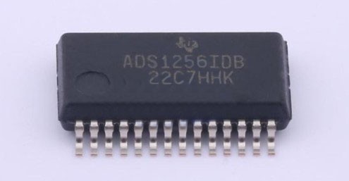 ADS1256
The ADS1256 is an high precision low noise 24-bit ADC. One of its biggest advantages is that it includes an internal Programmable Gain Amplifier (PGA) capable of amplifying the signal up to 64 times. It communicates via a SPI port.
This component is capable of sampling at a rate of up to 30,000 samples per second (SPS). However, there is always a trade-off between speed and noise resolution. The problem with measuring at such high speeds is that the output signal will contain a higher level of noise. Therefore, despite having the capability to go up to 30k SPS, we will configure the chip via software to use a more balanced sampling rate of around 2000 to 4000 SPS. This frequency is the middle point that allows me to capture the changes perfectly while maintaining a clean signal.
The hardware implementation of this chip is considerably more complex and rigorous than the classic HX711, as it requires extreme care regarding signal integrity and power supply quality. I have divided the schematic into two parts to make it easier to understand the function of each block:
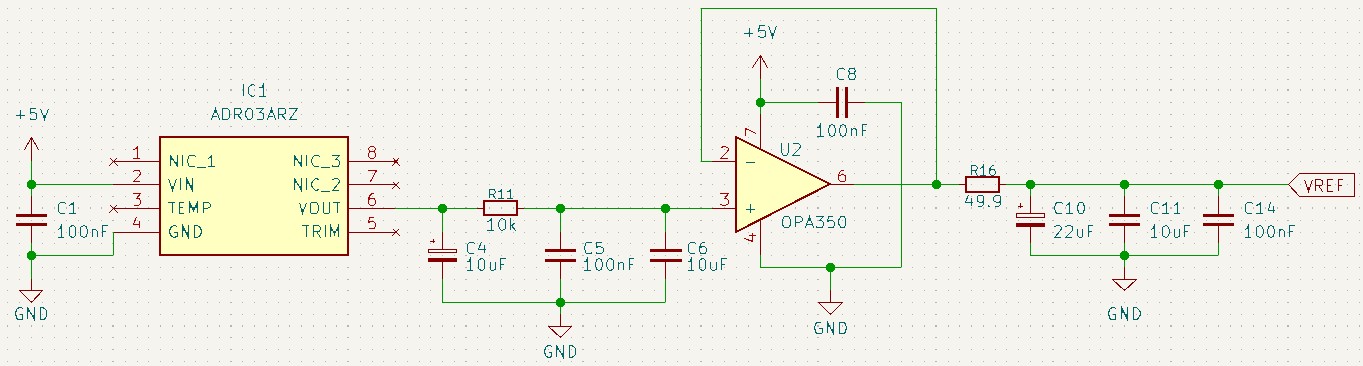 Voltage Reference
1. High Precision Voltage Reference (ADR03ARZ + OPA350)
An ADC works by comparing the sensor’s input voltage against an internal or external reference voltage. If that reference voltage fluctuates even slightly (due to temperature changes or bus loads), the ADC will interpret that noise as a change in the sensor value. For a 24-bit ADC, we cannot rely on the standard 5V supply as a reference.
In this design, a dedicated high-precision chip (IC1, ADR03ARZ) takes the 5V input and generates an stable 2.5V output. To ensure this reference remains stiff even when the ADC is switching its internal capacitors at high speed, I’ve added a precision Op-Amp (U2, OPA350) configured as a unity-gain buffer. The decoupling (C10, C11, C14) ensures the reference remains solid during instantaneous current demands.
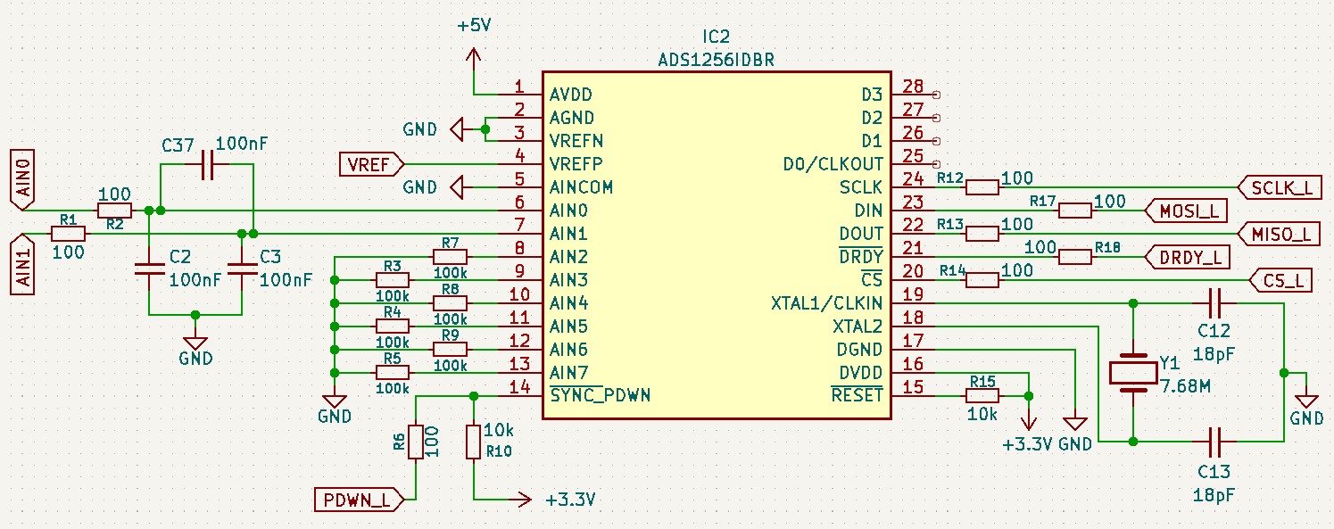 Main ADS1256 Schematic
2. Power Supply and Logic Levels
If we look at the power supply of the ADS1256 chip itself (IC2), there is a design detail: the analog section (AVDD) is powered at 5V, giving us the maximum possible dynamic range to read the sensor. However, the digital section (DVDD) is specifically powered at 3.3V.
By doing this, I force the SPI communication pins (CS, DIN, DOUT, SCLK) to operate natively at 3.3V. This matches the logic level of the Teensy 4.1 exactly, allowing me to connect both chips directly without the need of level shifters.
3. External Clock
To work precisely, the chip needs a very stable master clock. This is provided by an external 7.68 MHz quartz crystal (Y1) with 18pF load capacitors.
4. Anti-Aliasing Filters on Analog Inputs
In a dynamometer environment, load cell cables act as huge antennas, picking up electromagnetic interference (EMI). Before the differential signal enters the chip via AIN0 and AIN1, it goes through a passive RC filter:
- Common-mode filter: The capacitors connected to ground (
C2,C3) eliminate noise that affects both lines equally. - Differential filter: The capacitor connected directly between both signal lines (
C37) filters noise that exists between the lines.
Together, these form a hardware anti-aliasing filter. It ensures high-frequency noise is shunted to ground before the ADC attempts to sample the signal, guaranteeing that your torque readings are consistent and immune to shop noise.
This design had two big problems: The ADS1256 measured the load cell non-ratiometrically. The bridge was excited from the +5V rail produced by the XL1509 switching regulator, while the ADC’s reference came from a completely separate source, the fixed 2.5V from the ADR03 precision reference. Because a load cell’s output is proportional to its excitation and the ADC only measures the ratio of input to reference, the reading scaled directly with the absolute value of that 5V rail.
Also, a switching regulator’s DC output is neither perfectly stable, it shifts with line, load, temperature, and the startup transient so every power-up means a slightly different gain, which is exactly why the scale value had to be re-entered each time. The accuracy was perfect but a new calibration was necessary on every startup. This was not acceptable for this application.
Load Cell Amplifier (ADS1220)
As I mentioned earlier, the ADS1256 had a big problem in the current setup. After researching other alternatives, I decided to use the ADS1220 from Texas Instruments.
The ADS1220 design fixes this by tying the reference directly to the excitation: REFP0/REFN0 connect to E+/E− (the same rail that powers the bridge), so V_REF = V_EXC. On top of that, the excitation itself was moved off the switcher onto a dedicated low-noise linear LDO (the LT3045, on the separate +5VA rail), so the raw counts are quieter and stable.
 ADS1220
The ADS1220 is a high-precision 24-bit ADC. It includes an internal Programmable Gain Amplifier (PGA) capable of amplifying the signal up to 128 times. It communicates via an SPI port with the microcontroller.
This component is capable of sampling at up to 2 kSPS in “turbo mode” (1000 SPS base rate). There is always a trade-off between speed and noise: at the highest data rates the output contains more noise. I configured the chip via software to use turbo mode (effective 2 kSPS) with the internal FIR filter disabled.
The key configuration parameters used in this project are:
| Parameter | Value | Description |
|---|---|---|
| PGA | 128× | Maximum gain to amplify the very small differential signal from the load cell bridge. |
| MUX | AIN0–AIN1 (differential) | Differential input between channels 0 and 1. |
| Data rate | 1000 SPS turbo (2 kSPS) | Balanced speed/noise trade-off for this application. |
| VREF | External 5 V | A stiff external reference (the ADS1220’s own reference is not used). |
| FIR filter | Off | Internal 50/60 Hz rejection filter disabled; the firmware-side cascaded IIR handles all filtering. |
The hardware implementation of this chip is simpler than the ADS1256 alternative (which I considered initially). The ADS1220 does not need an external voltage-reference IC, an external buffer op-amp, or an external crystal, it uses the SPI clock and the external 5 V reference directly.
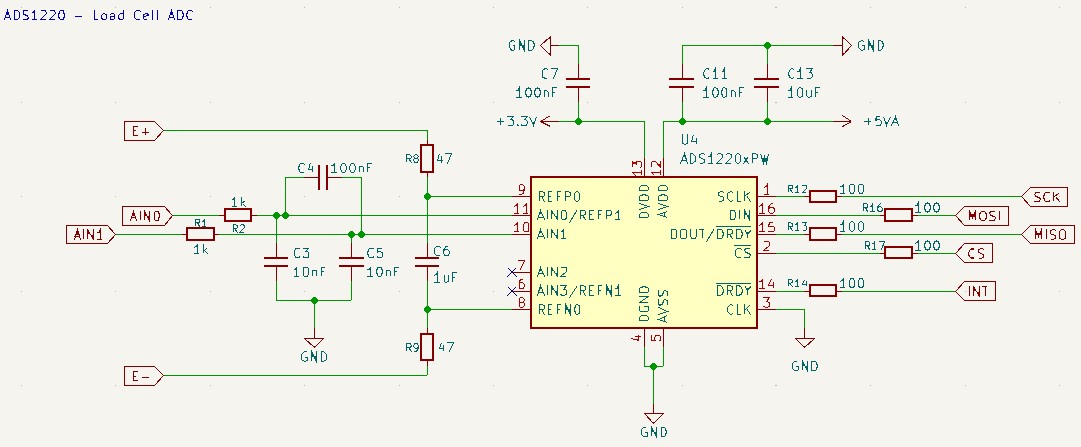 ADS1220 Schematic
An ADC never measures voltage in absolute terms, it measures the ratio between its input and its reference. In the previous design this worked against me, because the bridge was excited from one rail while the reference came from a separate fixed source, so any drift in the excitation was read as a change in torque. Here I turn that relationship into the fix. The reference pins of the ADS1220 (U4) are not tied to a fixed voltage at all: through the 47 Ω resistors R8 and R9, REFP0 and REFN0 connect straight to E+ and E−, the same rail that excites the load cell. Because a strain-gauge bridge’s output is proportional to its excitation and the ADC divides that output by the reference, the excitation term cancels out completely.
The reading now depends only on the physical force on the cell, not on the absolute value of the supply. This is a ratiometric measurement.
The differential pair from the cell enters through the series resistors R1/R2 (1 kΩ), with C4 (100 nF) bridged across the two lines to reject differential noise and C3/C5 (10 nF to ground) to shunt the common-mode interference picked up by the long load-cell cables.
The reference gets the exact same treatment, R8/R9 together with C6 (1 µF) across REFP0/REFN0 so signal and reference are filtered identically and stay locked together.
The chip then runs on a split supply: the analog side AVDD at 5 V (+5VA, decoupled by C11/C13) and the digital side DVDD at 3.3 V (C7) so the SPI lines drive the Teensy 4.1 directly without level shifting. Finally, tying the CLK pin to ground selects the ADS1220’s internal oscillator, so unlike the ADS1256 this stage needs no external crystal at all.
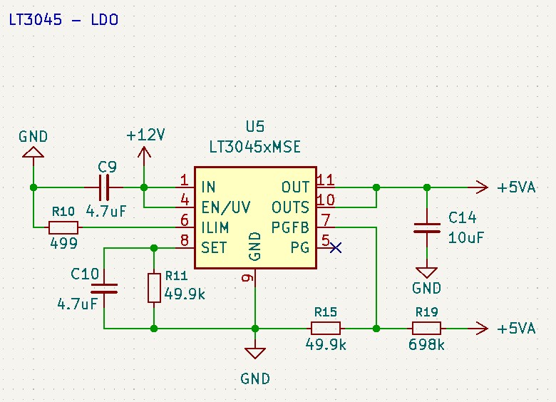 LT3045 LDO Schematic
A linear regulator has been chosen specifically for how quiet and stable it is. The LT3045 (U5) takes the +12V rail, decoupled by C9 (4.7 µF), with EN/UV tied to the input so it comes up the moment 1V is present and produces a clean +5VA.
The chip pushes a precise 100 µA out of its SET pin, so a single resistor to ground programs the voltage. Here R11 (49.9 kΩ) gives 100 µA × 49.9 kΩ = 5 V. That clean rail is exactly what the ratiometric scheme needs because the bridge excitation and the ADC reference both ride on it.
The R10 (499 Ω) on the ILIM pin programs the current limit, OUT (pin 11) and the Kelvin sense pin OUTS (pin 10) tie together at +5VA, with C14 (10 µF) holding the rail stiff against instantaneous current demand. Finally, R19 (698 kΩ) and R15 (49.9 kΩ) form a divider from the output into the PGFB pin.
Isolated ADC (MAX22530AWE)
Another feature I wanted to introduce was measuring the voltage at which the eddy current brake is operating. I could use one of the microcontroller’s internal ADCs for this, but we must remember that the eddy current brake can operate at around 325V. In the event of a back-EMF spike caused by the inductance of the coils, these transient voltages can reach up to 1200V. Connecting them directly to the microcontroller, even with basic protections, was simply not a safe option.
As we saw earlier, in the DynoPower board I used a voltage divider to step down the voltage to a manageable range. However, for this design, I wanted to guarantee the safety of the logic circuit by preventing voltage spike from ever reaching the board. To avoid short circuits and isolate the ground planes, I decided to use an external ADC with galvanic isolation. I had already used this approach in a previous electric motorcycle project, so I had some experience. The chosen component was the MAX22530AWE.
This specific ADC operates with a maximum voltage of 1.8V. Because of this, I had to be careful to ensure that, even in the worst scenario, the voltage reaching the chip’s input pins would never exceed that 1.8V limit.
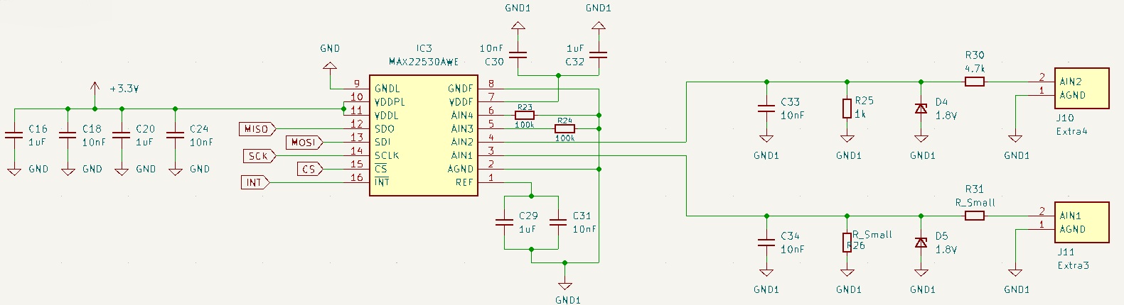 MAX22530AWE Schematic
The MAX22530 is a 12-bit ADC with 4 independent multiplexed channels capable of sampling at 20k sps. But the primary reasons were:
- Galvanic Isolation: The chip splits the high-voltage environment (DynoPower) and the low-voltage environment (DynoLogic).
- Integrated Isolated DC-DC Converter: Normally, to read an isolated sensor, you need to provide a separate power supply to power the high-voltage side of the ADC. This chip, however, includes its own internal DC-DC converter. It takes the 3.3V from our safe logic side and transfers the power across the isolation barrier to power its own reading circuitry on the high-voltage side.
If we break down the schematic, we can clearly divide it into two parts separated by the chip’s internal isolation barrier:
1. The Logic Side
This is the low voltage zone that connects directly to our Teensy 4.1.
- It is powered through the
VDDAandVDDDpins using the standard, clean 3.3V from our logic board. - Communication is handled via a standard SPI bus (
CS,SCLK,DIN,DOUT).
2. The Power Side
This is the high-voltage zone exposed to the eddy current brake.
- Self-Generated Power: The
VDDF(Field Power) pins are the output of the integrated DC-DC converter. As seen in the schematic, they require decoupling capacitors to filter and stabilize the voltage the chip just generated for itself. TheGNDFpin is the isolated ground. - Analog Inputs (
AIN1toAIN4): This is where I connect the signals coming from our voltage divider. I only use one signal but as I had 4 inputs available I wanted to leave one left for another use if necessary.
Temperature and Humidity Sensor (DHT11) (Deprecated)
 BME280
Another sensor I integrated into the board was the DHT11. This sensor allows the system to collect ambient temperature and humidity. Internally, it uses a capacitive humidity sensor and a thermistor returning the data through a single-wire serial bus.
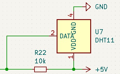 BME280 on I2C1
The 10k resistor (R22) between the 5V supply and the data line is a pull-up resistor. This is necessary because the DHT11 uses an open-drain communication protocol.
Finally, the DHT11 was not valid. Its single-wire protocol blocks the microcontroller. To work, it must measure the duration of each bit’s pulse in real time, which forces millisecond stalls in the main control loop. Even with non-blocking wrappers, the bit-reading phase cannot be deferred. This was locking the 1 kHz PID is running, so I replaced the DHT11 with the BME280.
Temperature and Humidity Sensor (BME280)
 BME280
For ambient temperature and humidity I use a Bosch BME280, connected on the Teensy’s secondary I2C bus (Wire1: SCL1 = pin 16, SDA1 = pin 17, address 0x76). The BME280 also reports barometric pressure, although the dyno only uses temperature and humidity.
The BME280 USES standard I2C. It can be polled in a background thread (via TeensyThreads) without disturbing the real-time loop. The chip’s internal IIR filter is disabled (Adafruit_BME280::FILTER_OFF); the dyno does not need sub-degree ambient accuracy.
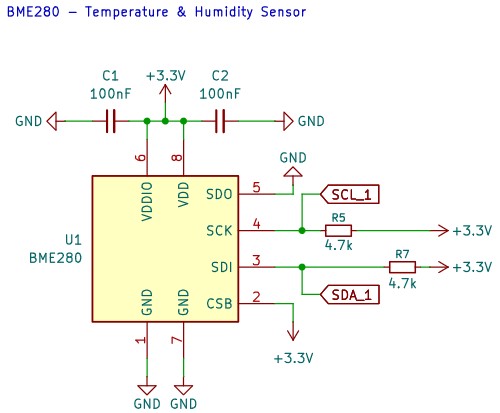 BME280 Schematic
The BME280 is read once per second from a background thread and the values are sent to DynoServer every 5 seconds via CAN 0x07.
PWM
To control the power delivered to the power stage (DynoPower), I use a PWM (Pulse Width Modulation) Signal. PWM allows a microcontroller to simulate an analog output using strictly digital signals.
It achieves this by switching a digital pin HIGH and LOW. The resulting square wave has two defining characteristics:
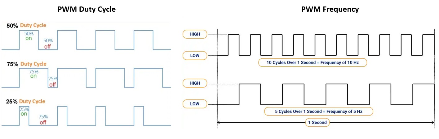 PWM Duty Cycle and Frequency8
- Frequency ($f$): This dictates how fast the entire HIGH/LOW cycle repeats, measured in Hertz (Hz).
- Duty Cycle ($D$): This is the percentage of time the signal remains HIGH during one period. If the signal is always ON, the duty cycle is 100%. If it is ON for half the time and OFF for half the time, the duty cycle is 50%.
By varying the duty cycle, we control the average voltage and power delivered to the load. A 50% duty cycle means the load sees 50% of the maximum available power.
In our power stage, the actual heavy lifting is done by power transistors (IGBTs). I feed the PWM signal to the IGBT. When the PWM signal is HIGH, the IGBT turns fully ON, acting like a closed switch and allowing the current to flow to the load. When the signal is LOW, it turns OFF, blocking the current.
However, there is a critical hardware problem we must solve: Voltage and Current.
The Teensy 4.1 operates at 3.3V. When the Teensy outputs a PWM signal, that HIGH state is only 3.3V, and the pins can only deliver few milliamps of current.
Power IGBTs cannot be driven directly by a microcontroller for two reasons:
- Gate Threshold Voltage ($V_{th}$): A 3.3V signal is not enough. To fully turn on an IGBT, the gate usually requires a voltage between 10V and 15V.
- Gate Capacitance: The gate of a large IGBT behaves like a capacitor. To turn the transistor on and off fast at high frequencies, you have to pump electrons into and out of that gate very fast. This requires short spikes of current (often several Amps). The Teensy’s cannot deliver that power.
This is exactly why the 15V rail and a gate driver are required. The Teensy sends its low-current 3.3V PWM signal to the gate driver. The gate driver then acts as a high-speed, high-current translator, using the 15V supply to charge and discharge the IGBT’s gate mirroring the microcontroller’s original PWM.
The Importance of Shielded Wires
After testing this feature, I encountered some issues. The PWM signal has an amplitude of 5V. If the wire is not shielded, the signal can degrade and look like this:
Invalid PWM Signal This signal does not reach the minimum threshold required by the gate driver to activate the IGBT.
Here is another example showing partial signal corruption:
Noisy PWM Signal
This issue is resolved by using a shielded wire. The shield must be connected to the GND side of the DynoLogic board only.
Level Shifter (TXS0108EPW)
There is an important compatibility consideration to keep in mind when connecting sensors to a microcontroller: the operating voltages.
The Teensy 4.1 microcontroller operates at 3.3V. This means that its digital inputs and outputs are designed for a maximum of 3.3V. If we accidentally inject a higher voltage into an input pin, we can damage the microcontroller.
On the other hand, many industrial sensors and modules operate at 5V. While some sensors are dual voltage, many still require a full 5V logic level to work correctly. This presents a problem: how do we connect a 5V sensor to a 3.3V microcontroller? This is where a level shifter comes in.
 TXS0108EPW
Essentially, a level shifter is an integrated circuit that translates digital signals between two different voltage domains, in this case, between 3.3V and 5V in both directions. While it is relatively simple to use a voltage divider to drop a 5V signal down to 3.3V, doing the opposite (boosting 3.3V to 5V) is more complex. Furthermore, many communication protocols are bidirectional, meaning the same wire carries data in both directions. A simple resistor network cannot handle this, but a chip like the TXS0108EPW can.
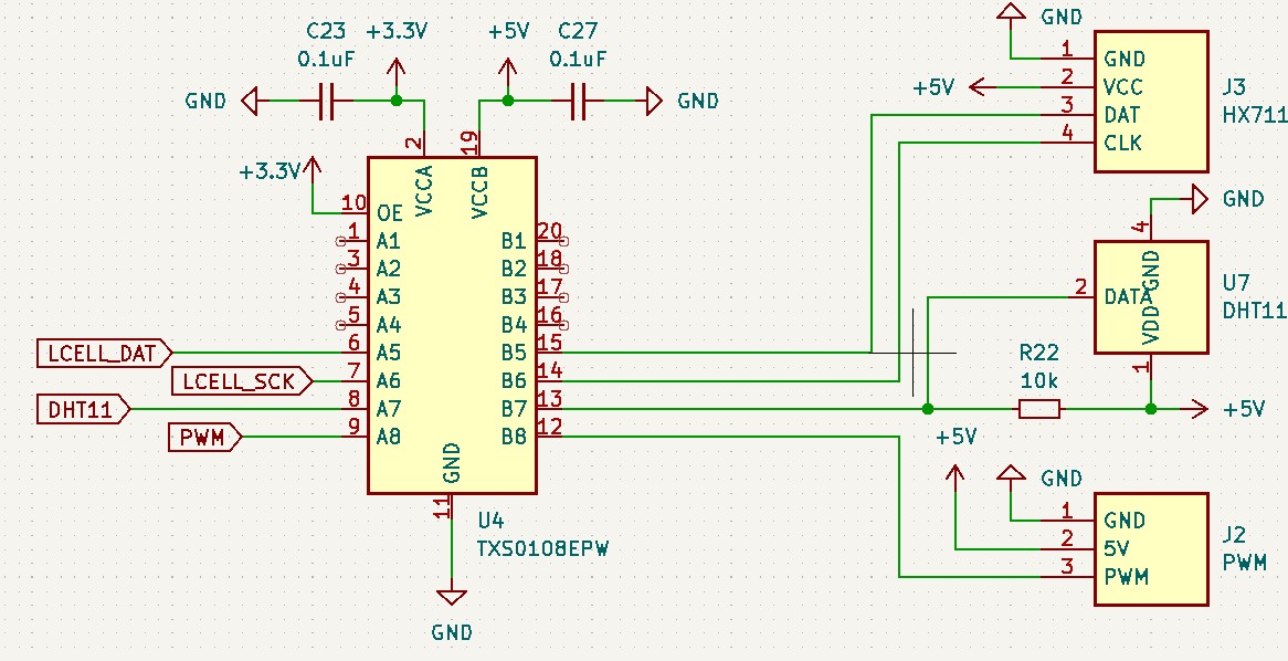 TXS0108EPW
In the schematic above, you can see that the HX711 (the alternative load cell amplifier) module operates at 5V, while the Teensy 4.1 stays at 3.3V. By placing the level shifter between them, each component operates at its native voltage while communicating perfectly. The default ADS1220 ADC and the BME280 are wired directly to the Teensy’s SPI0 and Wire1 buses at 3.3V, so they do not require the level shifter. We also use the level shifter to amplify the 3.3V PWM output signal from the Teensy to a 5V signal for the DynoPower board.
The only critical configuration step for the TXS0108EPW is connecting the OE (Output Enable) pin to the 3.3V rail to keep it active.
CAN-Bus
Another fundamental feature I needed to implement was communication between the logic PCB (DynoLogic) and the Raspberry Pi (DynoServer). For this, I evaluated different communication buses like I2C or UART, but CAN was the one that best fit my requirements.
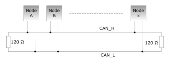 CAN Bus Topology9
The Controller Area Network (CAN) is a robust. It uses a serial bus originally designed for automotive applications. Its main advantage is its differential signaling (using two wires: CANH and CANL), which makes it extremely resistant to electromagnetic interference (EMI).
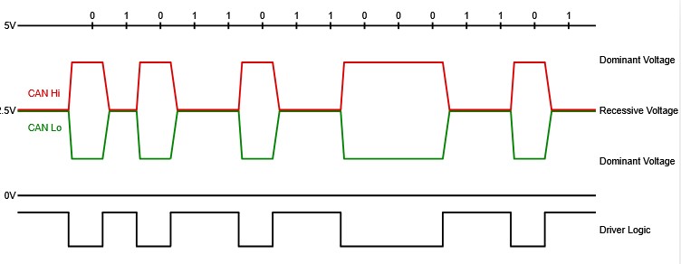 CAN Bus Signals10
To connect a device to a CAN network, the architecture typically requires two main hardware components:
- CAN Controller: Handles the protocol logic, message framing, error checking, and arbitration.
- CAN Transceiver: Acts as the bridge between the digital logic levels of the controller (TX/RX) and the differential physical voltage levels of the bus itself.
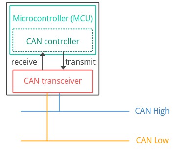 CAN Bus Architecture11
In my case, this CAN network would only have two nodes: DynoLogic and DynoServer. The Teensy 4.1 microcontroller features multiple internal CAN controllers. This greatly simplifies the integration, but we still need to add an external CAN transceiver to interface with the physical bus wires.
 SN65HVD230
For this, I decided to use the SN65HVD230. The main reason is that it operates at a 3.3V which perfectly matches the Teensy 4.1. If I had used another common transceiver like the 5V TJA1050, I would have needed to use the level shifter with it. That wouldn’t make much sense if a 3.3V transceiver is available.
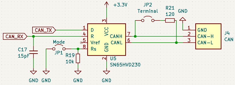 SN65HVD230 Schematic
Looking at the schematic, you can see the implementation is quite simple. The transceiver is powered at 3.3V. I included a jumper (JP2) in series with the 120-ohm termination resistor. Because the CAN standard specifies a 120-ohm characteristic impedance, this jumper must be active at both physical ends of the bus to ensure the network functions correctly.
Additionally, I included another jumper (JP1) for the mode selection. This jumper is connected to the $R_{S}$ of the transceiver to control its operating state. When the jumper is closed, the $R_{S}$ pin is pulled to ground, placing the transceiver in high-speed mode for maximum data rates. When the jumper is open, the pin connects to ground through a 10 kΩ resistor, placing the device into slope control mode. This mode artificially slows down the rise and fall slopes of the driver output which improves signal integrity.
Finally, there is a small 15pF capacitor on the receiver output (CAN_RX) to ground. This acts as a minor high-frequency noise filter, although it wouldn’t be strictly necessary for basic operation.
Beware of counterfeit chips.
I initially used some supposed SN65HVD230 transceivers from cheap breakout boards purchased from China, and the CAN bus simply did not work properly. I couldn’t get it to send or receive data correctly. After analyzing the bus with an oscilloscope, I observed the following:
Fake SN65HVD230 Waveform As you can see, the signal is heavily distorted and the data does not arrive correctly. The underlying issue with many of these counterfeit chips is that they are actually relabeled 5V transceivers (such as the TJA1050). When powered by the 3.3V supply of our logic board, they fail to generate the required 2V differential for the dominant state. Instead, they produce incorrect signals.
Below is an image of the exact same setup, but with a genuine transceiver:
Original SN65HVD230 Waveform With the original chip, the signal is clean and reaches the correct voltage levels.
IR Temperature Sensor (MLX90614)
Another critical aspect of this system is the temperature of the eddy current brake. All the energy it absorbs during braking is transformed into heat and dissipated through the rotors, making it an important element to monitor.
Because the rotors are moving parts spinning at thousands of revolutions per minute (RPM), using a traditional contact temperature sensor (like the DS18B20 or a standard thermistor) was impossible. Instead, I decided to use a non-contact infrared (IR) temperature sensor, specifically the MLX90614, which you can see below:
 MLX90614
Every physical object emits infrared radiation (thermal energy) proportional to its temperature. The MLX90614 works by capturing this invisible light.
It outputs the temperature over a I2C digital bus (using the SDA and SCL lines).
I made a hardware modification to this sensor module. The commercial boards for the MLX90614 (often labeled GY-906) typically include a linear voltage regulator (LDO). This regulator is designed to take a 5V input and step it down to the 3.3V required by the bare sensor chip.
While you can supply 3.3V directly to the module, forcing that voltage through the regulator introduces a small voltage drop. The sensor ends up receiving slightly less than 3.3V. I decided to remove the module’s regulator. By bridging the pads, the 3.3V power from the DynoLogic board feeds directly into the sensor chip.
DS18B20 Temperature Sensor
Although the components used in the DynoPower board are significantly oversized and shouldn’t present any thermal issues, I wanted to include a temperature sensor to actively monitor the system and ensure nothing overheats under heavy loads. For this, I decided to use a DS18B20 sensor that I already had on hand.
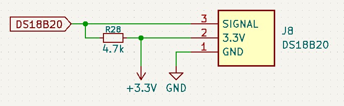 DS18B20
These temperature sensors communicate using the One-Wire protocol. This protocol only requires a single data line (and GND) to establish communication with the microcontroller.
Additionally, the One-Wire bus relies on an open-drain configuration. This means it requires a pull-up resistor (4.7kΩ) connected between the data line and the VDD supply line. This resistor ensures the bus returns to a stable HIGH state when no device is transmitting data, preventing noise and communication errors.
Power Supply
The DynoLogic board is powered by an external 12V DC source (typically from a 230VAC to 12VDC adapter). In my experience, it is only a matter of time before someone plugs the connector in backwards, so the very first thing the 12V meets on the board is reverse-polarity protection.
In the first version of the board I solved this with a bridge rectifier at the DC input. A single series diode would have been enough to block reverse current, but a bridge rectifier goes one step further: it makes the input polarity-agnostic, so the board powers up correctly regardless of which way the two 12V wires are connected.
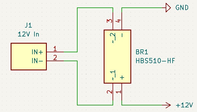 HBS510-HF
The downside is the forward voltage drop. Current always passes through two of the bridge’s diodes, so it loses roughly $V_f \approx 1.2\text{V}$ to $1.4\text{V}$. Starting from 12V that still leaves about $\approx 10.6V$, which is enough to feed the regulators and the 12V encoder, but it is wasted voltage, and that drop turns into heat that grows with load current.
In the current design I replaced the bridge with a P-channel MOSFET (U2) acting as an “ideal diode”. Unlike a rectifier, a MOSFET conducts through its channel resistance ($R_{DS(on)}$) of just a few tens of milliohms. The 12V input feeds the drain, the protected +12V rail is taken from the source, and the gate is pulled down to ground through R6 (10k).
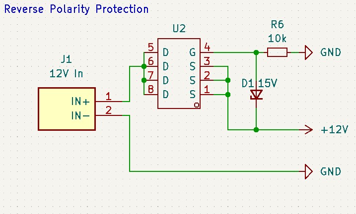 Reverse Polarity Protection
When the supply is connected the right way around, the gate sits at ground while the source sits near +12V, so $V_{GS}$ is strongly negative and the P-channel turns fully on. Current then flows through that tiny $R_{DS(on)}$ and the drop across the device is only millivolts, so practically the entire 12V reaches the regulators. If the supply is reversed, the source can no longer rise above the gate, $V_{GS}$ collapses to zero and the MOSFET stays off; its internal body diode is reverse-biased in that case as well, so it blocks too, and no current flows into the board at all.
D1, a 15V Zener wired across gate and source, clamps $V_{GS}$ to a safe level so the thin gate never sees the full input voltage or a transient spike, and R6 does double duty, it pulls the gate low to switch the FET on, and it limits the current through the Zener whenever it clamps.
5V Power Supply
While the input is 12V, the Teensy 4.1 and several sensors require a stable 5V rail. When choosing a regulator, there are two main contenders: LDOs (Linear Regulators) and Buck Converters (Switching Regulators).
LDOs vs. Switching Regulators
- LDO (Linear Low Dropout): These are essentially electronically controlled resistors. They are very simple and provide a clean output with no switching noise. However, they are inefficient. They dissipate the voltage difference as heat. In this case, dropping from 12V to 5V at a “high current” would make the regulator get hot.
- Switching Regulator (Buck Converter): These work by “chopping” the input voltage and using an inductor to smooth it. They are efficient (often >90%). The downside is that the high-frequency switching can introduce electrical noise into the circuit.
Given the current requirements of the Teensy 4.1 and all the peripheral sensors, I chose the XL1509-5.0 switching regulator to avoid heat management issues.
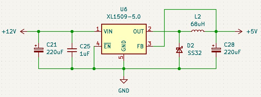 XL1509-5V
Circuit Breakdown:
- Input Stage: The regulator takes the main 12V DC input from the bridge rectifier.
- The Regulator: The XL1509-5.0 handles the high-frequency switching to step the voltage down.
- Output Filtering: According to the datasheet, the 5V version typically requires a 180uF output capacitor for stability. However, to simplify the BOM and match the 3.3V rail, I standardized on a 220uF capacitor. This acts as a middle point that satisfies the stability and ripple-filtering for this load.
3.3V Power Supply
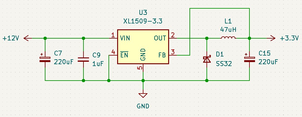 XL1509-3.3V
To supply the 3.3V rail required by the Teensy 4.1’s core and other low-voltage peripherals, I implemented a second switching regulator circuit using the XL1509-3.3.
Notice that instead of chaining this regulator off the 5V output, it is powered directly from the main 12V input. This parallel configuration is a deliberate design choice: it distributes the total power dissipation and current load across two separate ICs, rather than forcing the 5V regulator to work twice as hard to power the entire board.
Circuit Breakdown:
- Input Filtering: The 12V input is stabilized by a 220µF electrolytic capacitor (
C7) to handle low frequency power surges paired with a smaller 1uF capacitor (C9) to bypass high-frequency noise before it enters the IC. - The Regulator (U3):(
ENor Enable) is tied directly to ground. Because this is an active-low pin, this ensures the 3.3V rail turns on immediately and stays on as long as the board has power. - The Switching Core: The 47uH inductor (
L1) and the SS32 Schottky diode (D1) maintain the current flow to the load. The SS32 diode provides the necessary return path (freewheeling diode). - Output Filtering: The output is smoothed by a 220uF capacitor (
C15).
Onboard LED
I also added a LED to check if DynoLogic was turned on.
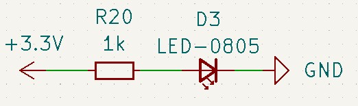 3.3V LED
For this specific 0805 SMD LED (D3) connected to the 3.3V line, the circuit uses a 1kΩ current-limiting resistor (R20).
I can calculate the forward current ($I_f$) flowing through this LED using Ohm’s Law as done previously. Assuming it has the same forward voltage ($V_f$) of roughly 2.3V as the other indicators:
\[I_f = \frac{V_{in} - V_f}{R}\] \[I_f = \frac{3.3V - 2.3V}{1000\Omega} = \frac{1.0V}{1000\Omega} = 0.001A = 1mA\]Versions
Not everything works out the first time, especially if you don’t know what you’re doing. Despite having made more than two PCBs (I don’t remember exactly how many), I can mainly distinguish two versions: v1, which used the Atmel SAM3X8E, and v2, which uses the Teensy 4.1.
DynoLogic v1
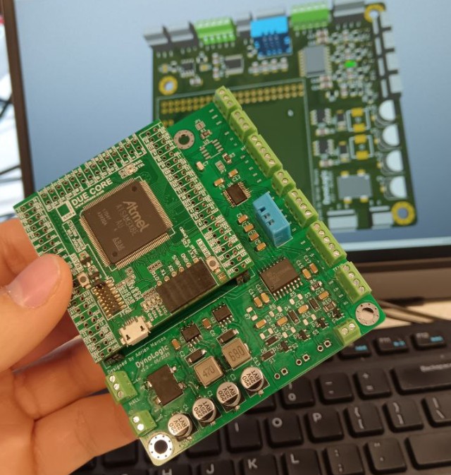 DynoLogic v1 using Atmel SAM3X8E
This board had some troubles with the i2c peripherals and used an older microcontroller.
DynoLogic v2
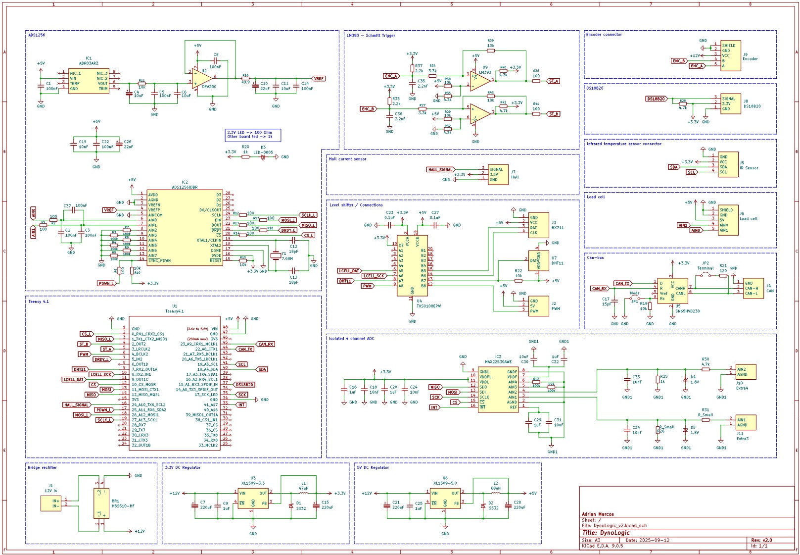 DynoLogic v2: Schematics
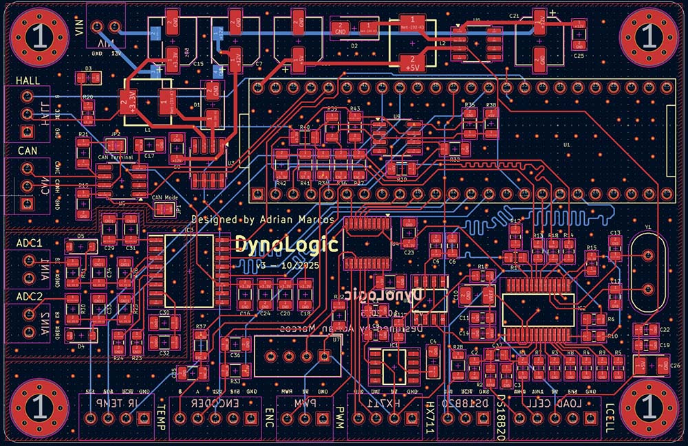 DynoLogic v2: PCB Design
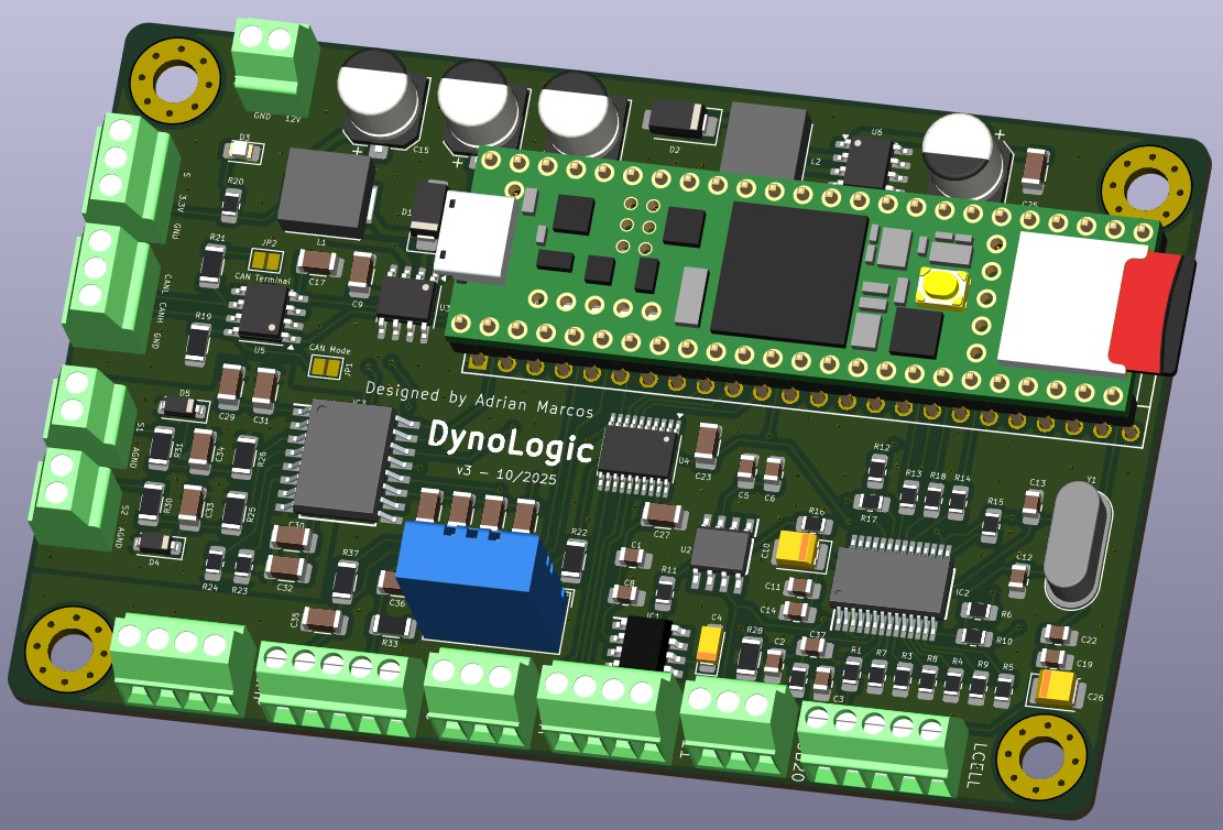 DynoLogic v2: 3D Render
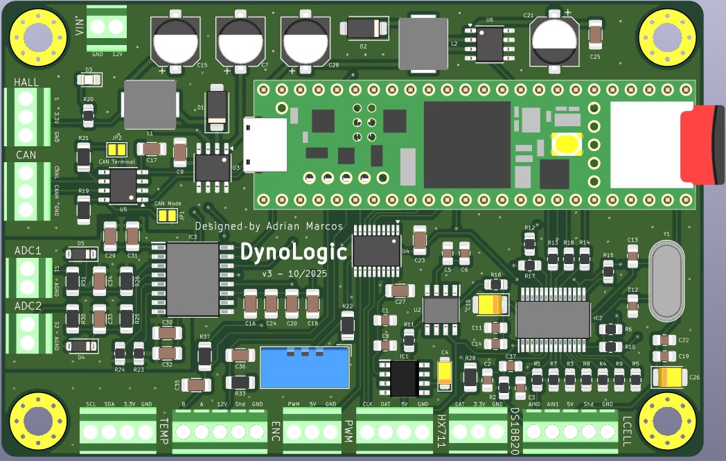 DynoLogic v2: Front View
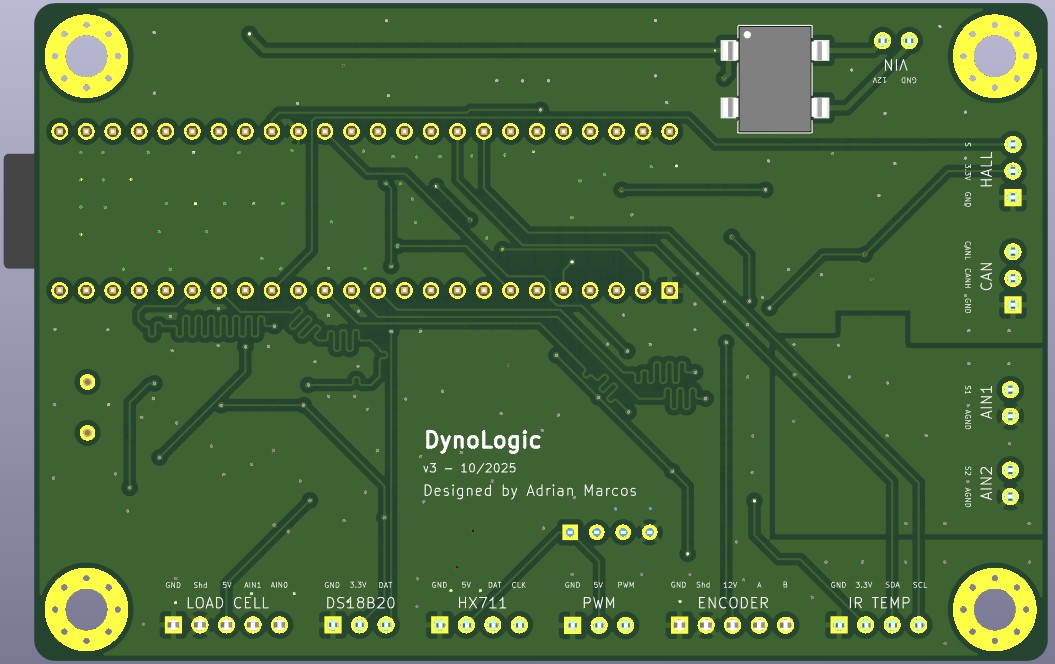 DynoLogic v2: Back View
This version was working correctly except because the load cell ADC needed a calibration on every startup. It was fixed in the v3 and also, the bridge rectifier at the input was replaced with a PNP MOSFET to protect the board from reverse polarity.
DynoLogic v3 - Current Version
This is the board currently in use
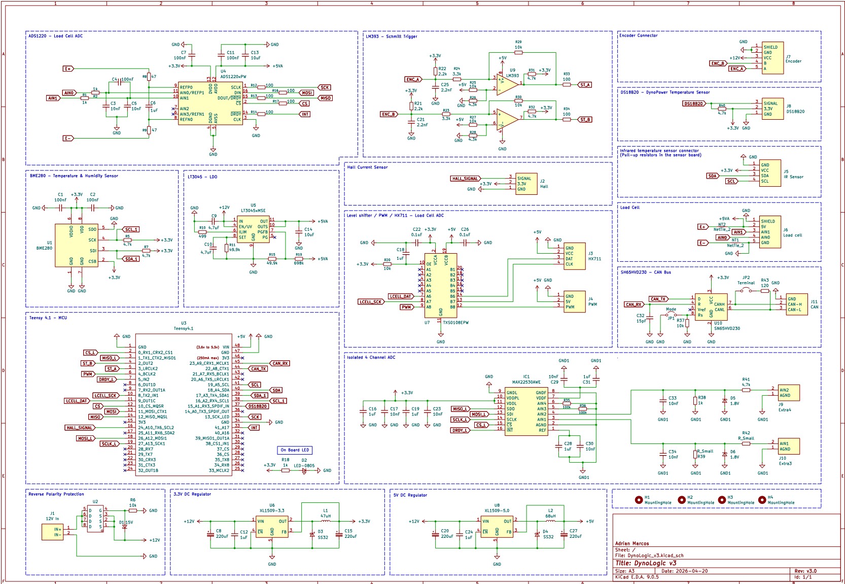 DynoLogic v3: Schematics
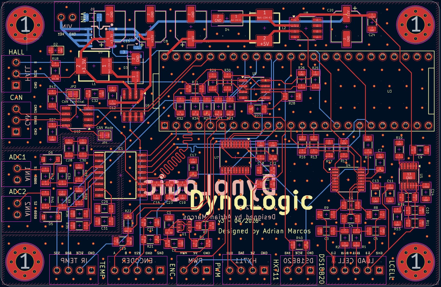 DynoLogic v3: PCB Design
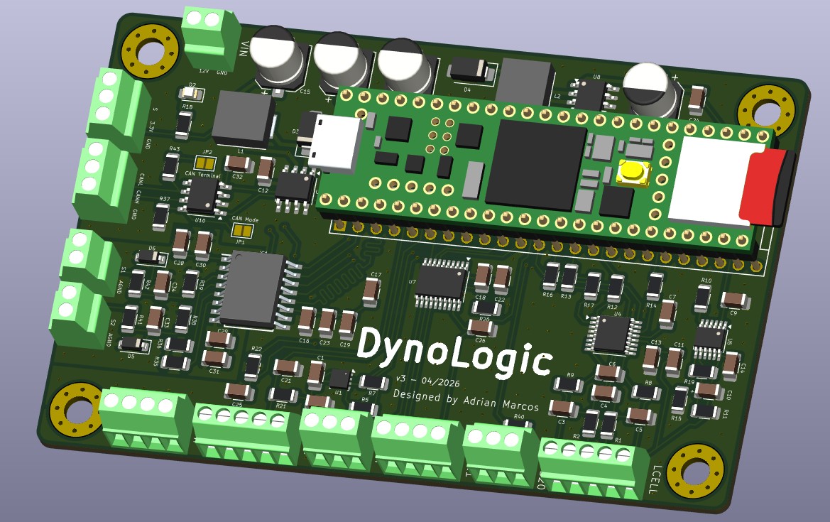 DynoLogic v3: 3D Render
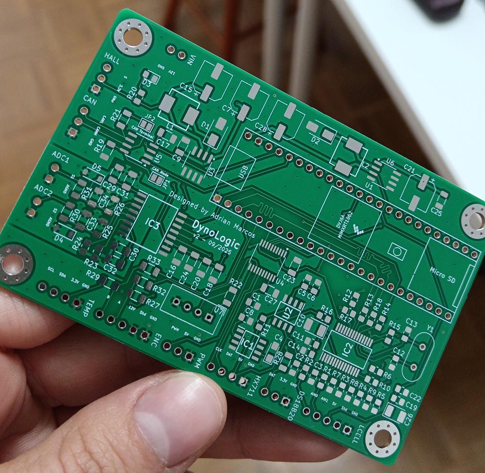 DynoLogic v2: Empty PCB
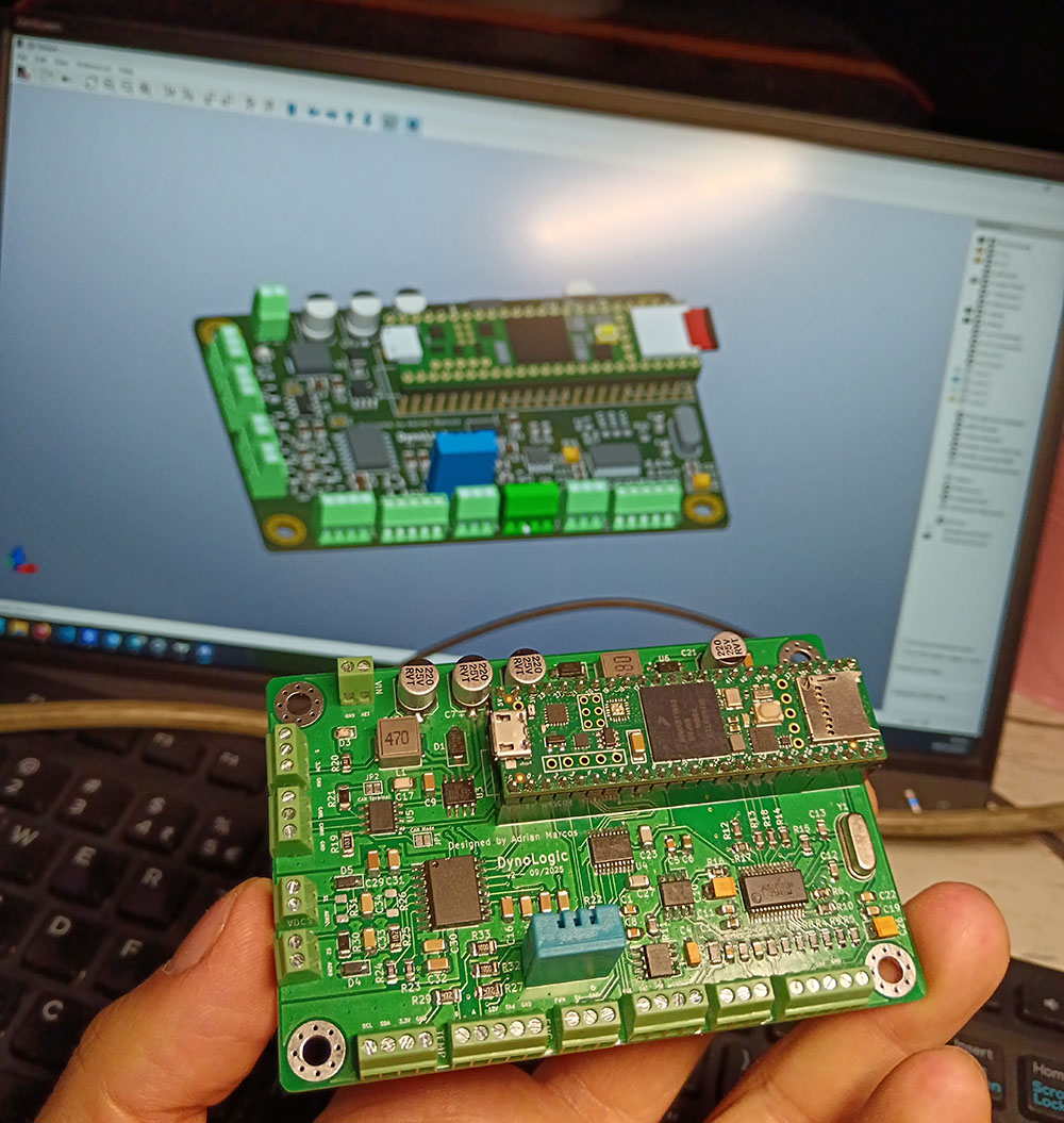 DynoLogic v2: Finished PCB
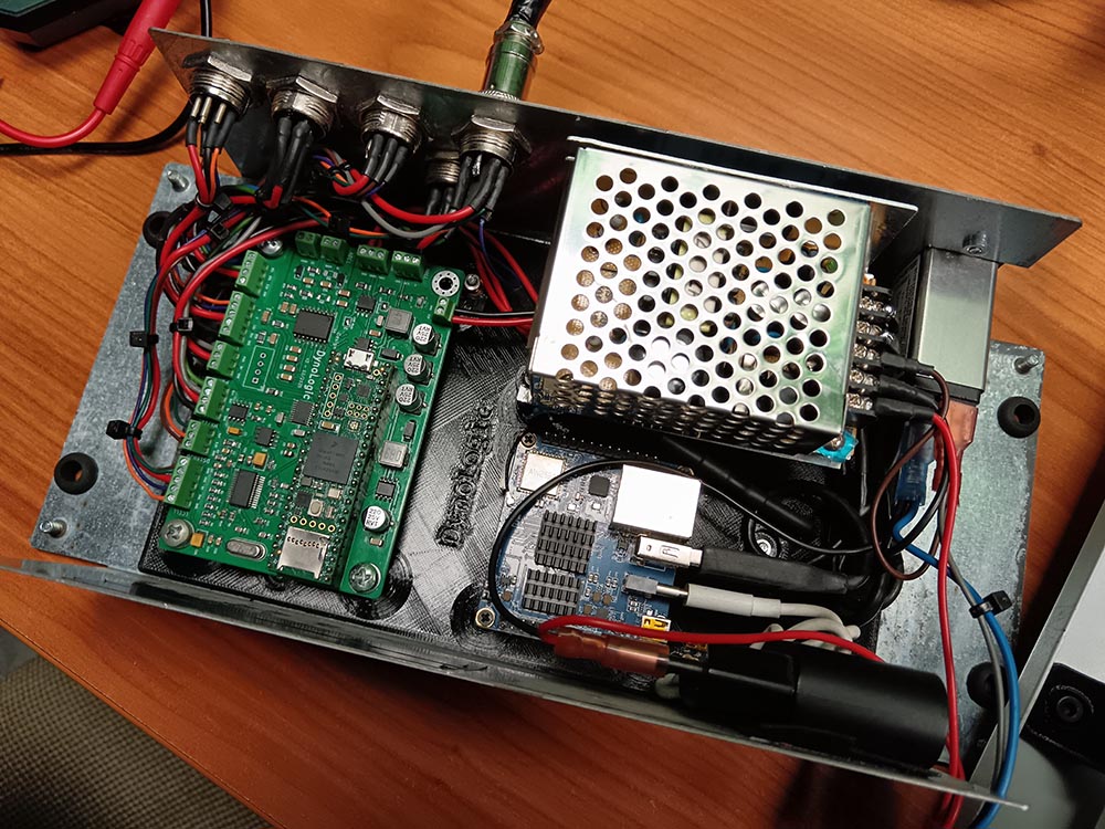 DynoLogic v2: Placed with the Orange Pi and CAN Interface
Finally, I used a CANable interface between the CAN interface of the Teensy 4.1 and the Orange Pi as it doesn’t have a CAN transceiver. I connected it into a USB port.
Software 💻
Let’s move on to another of the most complex phases of the project: everything related to software development.
As seen previously, here is the high-level architecture I designed for the system:
System Architecture
When considering how the user would interact with the system, I evaluated three options:
- A desktop application directly connected to the control board (DynoLogic).
- A remote computer (a Raspberry Pi, for example) connected to the control board and accessed via RDP or a similar remote desktop protocol.
- Web technologies using a client-server architecture.
The option I liked least was the second one, as I find it impractical for modern applications. While the first option was viable, I wanted to prioritize flexibility and cross-platform accessibility, so I decided to go with the 3rd option.
With this decision made, it was time to start the software development. Another critical choice was determining which communication protocols to use. We had already established that a PWM signal would handle the IGBT between DynoPower and DynoLogic. However, I now needed to analyze the most suitable protocol for communication between DynoLogic and the web server, which we will call DynoServer from now. As mentioned previously, I evaluated using UART and other protocols but finally I selected CAN.
For the server hardware, I chose a Raspberry Pi (specifically, an Orange Pi I had available) to be mounted inside the same physical enclosure as the DynoLogic board. This setup allows the system to be accessed seamlessly via both Ethernet and Wi-Fi.
Finally, the last major decision was how to transmit real-time data from DynoServer to the browser for the user interface. After some research, I decided to use WebSockets. Although I had never worked with this technology before, it looked like the perfect solution for this application, providing the low-latency updates required for live readings.
Working Modes
Let’s focus on the firmware development. The DynoServer application will be used as middleware between the user and the DynoLogic board, but the DynoLogic board implements all the logic of the system.
Going back to the main purpose of the system, we need to remember first what we want to do with it.
My initial idea was to have 4 working modes in the dyno. There could be an interesting 5th mode named “Track Mode” or “Simulation Mode” and with the correct telemetry I could be able to simulate a track or a dynamic situation. Unfortunately I didn’t have a good telemetry example of a real track lap so I didn’t develop this mode. The developed modes were:
Speed Mode
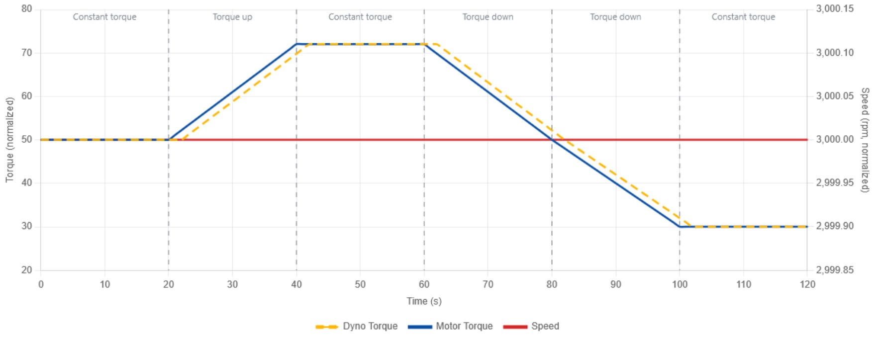 Speed Mode
In this mode, the dyno controls the speed of the motor. This means that the dyno will brake the motor and control it based on a specified speed. To do it the dyno will try to control the speed with a variable torque. As it’s shown in the graph, if the motor torque and the dyno torque are equal, the speed will remain constant. If the motor torque increases (you are accelerating), the dyno brake will increase too trying to keep the speed constant (and increasing the measured torque). If on the other side the motor torque is reduced, the dyno brake will be reduced too avoiding to brake too much the motor and making the speed drop.
Torque Mode
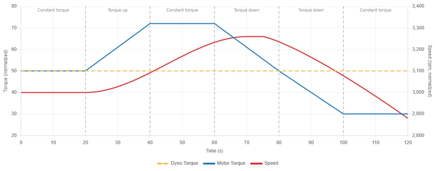 Torque Mode
In this mode, the dyno controls the torque of the motor. This means that the dyno will keep the desired torque constant. As it’s shown in the graph, if the torque of the motor and the torque of the dyno are equals, the speed will remain constant, like in the previous mode. The difference is when we accelerate the motor (increasing its torque), the dyno will keep brake torque constant so the speed will be increased. This will happen when the motor torque is higher than the dyno torque. If the motor torque drops below the dyno set torque then the speed will start decreasing.
Acceleration Mode
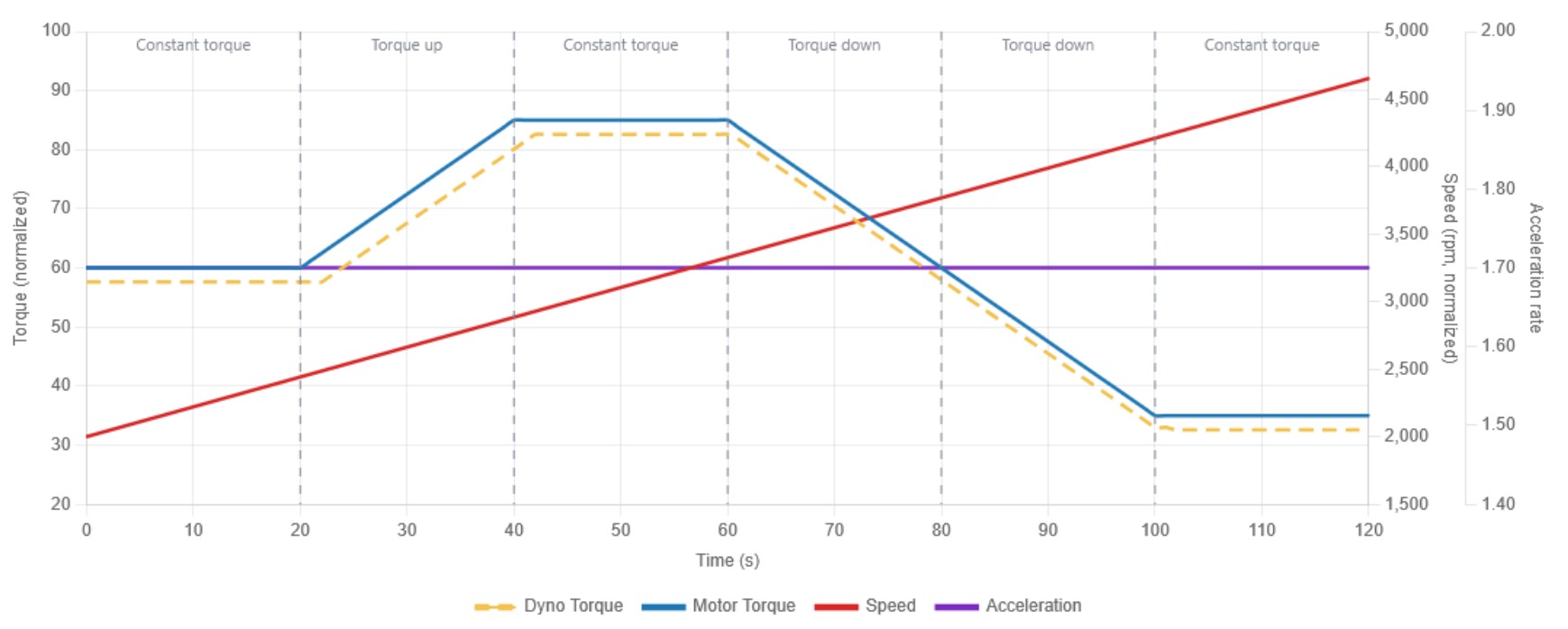 Acceleration Mode
In this mode, the dyno controls the acceleration of the motor. This means that the dyno will keep the desired acceleration measured in $RPM/s$. The dyno will limit at which rate the motor can accelerate. As it’s shown in the graph, to produce an acceleration the motor torque must be always bigger than the dyno brake torque. If the motor torque is increased the dyno will increase its brake torque too allowing the system to keep the desired acceleration (it will be always a bit lower than the motor torque). If the motor torque drops, the dyno brake will drop too trying to keep the necessary difference to keep the acceleration constant. As it’s shown, the purple line shows the acceleration, constant during the test and the speed increasing linearly because of the acceleration of the system.
Dynamic Mode
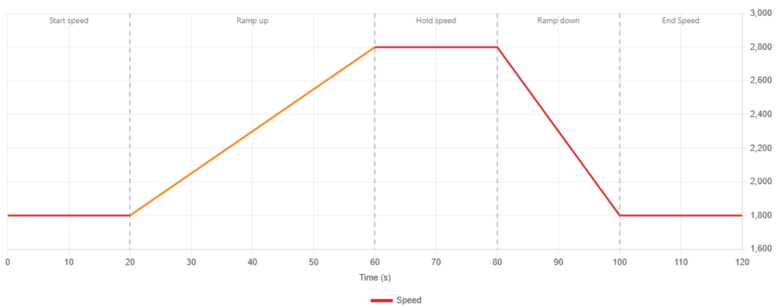 Dynamic Mode
In this mode, the dyno will iterate over different modes in the following stages:
- Start speed: During this stage, the dyno will work in speed mode trying to control the start speed of the test avoiding high torque changes.
- Ramp up: At this stage, the system will change to acceleration mode. In this stage the torque and speed measured is performed until it reaches the maximum defined speed.
- Hold Speed: Here, the system will change again to speed mode. This stage will allow the system to limit the maximum speed and avoid damage in the system or the motor. Once a torque drop is detected it will change to the next mode.
- Ramp down: This mode will brake the system to a lower speed to stop it.
- End speed: This will be the speed at which the system will stop braking the motor. This allows also the cooling of the eddy current brake.
This mode is the best-known one, where torque and power curves are produced. With these core concepts settled, we can now shift our focus to the software development.
DynoLogic
The microcontroller is programmed in C++. In the following sections, I will explain the firmware development step-by-step. The first stage involves data acquisition from the various sensors used by the system, such as the encoder, the load cell, and temperature sensors. The second stage focuses on the actuator, in this case, the PWM control and finally, the control logic implemented to achieve the system’s goals.
General Requirements
The primary requirement for this software is that it must operate in real-time. This means the code must be deterministic, with no blocking delays that could compromise the stability of the control loops.
As mentioned earlier, the system is designed around four well-defined operating modes: Speed, Torque, Acceleration and Dynamic.
Firmware
Execution Flow
This section provides a high-level overview of how the firmware executes, from power-on to steady-state operation. The entire system follows a classic microcontroller pattern, a one-time setup() followed by an infinite loop() function.
Startup Sequence
When the Teensy 4.1 powers on, the setup() function initializes all hardware peripherals in a deliberate order.
flowchart TD
    A["Power On"] --> C["PWM Initialization"]
    C --> D["Data Structures Initialization"]
    D --> E["PID Initialization"]
    E --> F["Timer Initialization"]
    F --> G["CAN Bus Initialization"]
    G --> H["Encoder Initialization"]
    H --> I["Load Cell Initialization"]
    I --> J["External ADC Initialization"]
    J --> K["IR Temp Sensor Initialization"]
    K --> L["DS18B20 Initialization"]
    L --> M["Hall Sensor Initialization"]
    M -->     N["BME280 Initialization"]
    N --> O["Status LED Initialization"]
    O --> P["Enter loop()"]

    style A fill:#2d2d2d,stroke:#6ee7b7,color:#fff
    style P fill:#2d2d2d,stroke:#6ee7b7,color:#fff
After setup() completes, the system enters loop() with all PIDs in manual mode (disabled), status set to STOPPED, and PWM at 0%. The microcontroller will not actuate the brake until it receives a valid configuration from the server and the START command.
Main Loop Architecture
The loop() runs as fast as possible. Each iteration executes two classes of work: continuous tasks that run every iteration, and scheduled tasks that run at specific rates set by the timer ISR.
Continuous tasks
- Sample Hall sensor
- Sample speed (encoder)
- Sample torque (load cell)
- Read DS18B20 state machine
- CAN: Check RX buffer
- CAN: Drain TX queue
- CAN: Parse received messages
- Configuration sync
- Connection watchdog with DynoServer
- Disconnect failsafe handling
- Update LED pattern
Scheduled tasks
These tasks run only when their corresponding timer flag is triggered.
| Task | Interval | Frequency | Description |
|---|---|---|---|
| Run PID controller | 1 ms | 1000 Hz | PID Control Loop |
| Send telemetry (speed, torque, acceleration) | 10 ms | 100 Hz | Send data to DynoServer |
| Heartbeat and electrical data | 100 ms | 10 Hz | System monitoring |
| Broadcast system status | 500 ms | 2 Hz | General system state |
| Send temperatures (DS18B20) | 1000 ms | 1 Hz | DynoPower Temperature Reporting |
Communication Lifecycle
The following diagram shows the communication lifecycle between the microcontroller and the server. It starts from the first connection, then a configuration request is done (because of invalid checksum), then the system is started and then stopped.
sequenceDiagram
    participant MCU as DynoLogic
    participant SRV as DynoServer

    Note over MCU: Power on → setup()

    MCU->>SRV: Heartbeat
    SRV->>MCU: Heartbeat
    Note over MCU: status.connected = true

    SRV->>MCU: Checksum
    Note over MCU: Mismatch → request config

    MCU->>SRV: Request Config
    SRV->>MCU: Configuration
    SRV->>MCU: Checksum
    Note over MCU: Match → valid_checksum = true

    SRV->>MCU: Run Mode + Setpoint
    SRV->>MCU: START Command
    Note over MCU: status = RUNNING, PID active

    loop Every loop iteration
        MCU->>MCU: Read sensors → Filter → PID → PWM
    end

    loop Every 10 ms
        MCU->>SRV: Speed + Torque + Timestamp
        MCU->>SRV: Acceleration + Timestamp
    end

    loop Every 100 ms
        MCU->>SRV: Heartbeat
        MCU->>SRV: Current + Voltage
    end

    loop Every 1 s
        MCU->>SRV: Brake Temperature
        MCU->>SRV: Ambient Temperature
    end

    SRV->>MCU: STOP Command
    Note over MCU: status = STOPPED, PWM = 0
Data Structures
All system state is organized into a small number of C structures defined in datatypes.h. This design centralizes all data that can be passed by reference to functions and serialized over CAN. There are two principal structures:
Configuration
This structure holds every tunable parameter of the system. It is received from the server application via CAN bus and its integrity is verified using a CRC-16 checksum. Both the microcontroller and the server must agree on the exact checksum. It has the following information:
| Sub-structure | Fields | Purpose |
|---|---|---|
pid_data (×3) |
kp, ki, kd |
PID gains for torque, speed, and acceleration controllers |
Run_mode |
mode, value |
Control mode and its setpoint |
Load_cell |
gain, offset, scale, distance |
Load cell calibration and lever arm length |
Pwm_config |
pwm_start, pwm_limit, pwm_frequency |
PWM safety limits and configuration |
Low_pass_filters |
speed, torque, acceleration, pid_output |
LP Filter Configuration |
Speed_limits |
min_speed, max_speed |
RPM Limits |
Dynamic_config |
start_speed, accel_rate, end_speed, etc. |
Dynamic mode parameters |
1
2
3
4
5
6
7
8
9
10
11
12
13
14
struct config
{
    uint8_t debug_mode;
    pid_data torque_pid;
    pid_data speed_pid;
    pid_data dynamic_pid;
    Run_mode mode;
    Load_cell load_cell;
    Pwm_config pwm_config;
    Low_pass_filters low_pass_filters;
    Speed_limits speed_limits;
    Dynamic_config dynamic_config;
};
typedef struct config Configuration;
The Configuration structure is never modified by the microcontroller itself. It is only written to when a CAN message from the server updates a specific field.
The normal workflow of this struct is:
- A parameter is changed in the DynoServer application.
- When the checksum is received by DynoLogic, it checks that it has an invalid configuration.
- It requests the new configuration.
- DynoServer sends back the whole configuration struct and the new checksum.
This is for every parameter except for PID Gains (Kp, Ki, Kd). When they are updated in the DynoServer application, they are sent directly to the DynoLogic so it’s not always required to send the whole configuration struct again.
Status
The Status structure holds everything the microcontroller produces (sensor readings, outputs, system state) and more. It is read by CAN functions to send telemetry to the server.
Many of its elements are declared volatile because they are written from interrupt context (encoder ISRs update speed, the timer ISR indirectly triggers updates) and read from the main loop.
TimeControl
This structure serves as the interface between the hardware timer ISR and the main loop. Each field is a pending-task counter that the ISR increments and the main loop consumes. It also tracks missed ticks.
1
2
3
4
5
6
7
8
9
10
11
12
struct time_control
{
    volatile uint8_t pending_1ms = 0;
    volatile uint8_t pending_10ms = 0;
    volatile uint8_t pending_100ms = 0;
    volatile uint8_t pending_500ms = 0;
    volatile uint8_t pending_1s = 0;
    volatile uint8_t pending_5s = 0;
    volatile uint32_t missed_1ms = 0;
    volatile uint32_t missed_10ms = 0;
    // and more
};
Hall Current Sensor
The hardware implementation of this sensor has been explained previously. It is connected to an ADC input of the Teensy 4.1. This sensor does not directly provide current in amperes, it outputs a voltage that must be converted into current.
We must take into account the specific characteristics of this model, the ACS781LLRTR-050U-T:
- Type: Unidirectional
- Sensed Current Range (IP): 0 to 50 A
- Sensitivity (Sens): Typical 39.6 mV/A (or 0.0396 V/A)
- Quiescent Output Voltage ($V_{OUT(QU)}$): This is the zero offset. For unidirectional models, it is 0.1 × $V_{CC}$. As we are supplying it at 3.3 V, this is 0.33 V.
Based on the datasheet, let’s calculate the formula to get the current based on the voltage:
The output voltage ($V_{OUT}$) of the sensor is proportional to the current ($I$). The relationship is defined as:
\[V_{OUT} = V_{OUT(QU)} + (Sens \times I)\] \[I = \frac{V_{OUT} - V_{OUT(QU)}}{Sens}\]Using the sensitivity of 39.6 mV/A (0.0396 V/A) for this model and the $V_{OUT(QU)}$ calculated previously:
\[I = \frac{V_{OUT} - 0.33 \text{ V}}{0.0396 \text{ V/A}}\]This is the formula we need to use. However, there is a critical challenge when measuring this specific application. We are measuring pulsating current, not DC. If we apply 1% of brake (1% PWM duty cycle at 1 kHz), the IGBT switches on for just 10 microseconds, followed by 990 microseconds where the current is strictly zero. If we just sample the ADC at random intervals, there is a 99% probability that we will sample during the OFF state, resulting in a false 0.0A reading.
To solve this, we cannot rely on random main loop sampling. Instead, the ADC sampling is hardware-synchronized using the FlexPWM interrupts.
First, we use a struct to store the accumulated measures for block averaging to reduce sensor thermal noise.
During system initialization, we configure a hardware interrupt linked directly to the PWM peripheral controlling the IGBT:
1
2
3
4
5
    // Configure FlexPWM hardware trigger for ADC synchronization
    // Attach to FlexPWM2 Submodule 0 (controls Pin 4)
    attachInterruptVector(IRQ_FLEXPWM2_0, flexpwm2_0_isr);
    NVIC_ENABLE_IRQ(IRQ_FLEXPWM2_0);
    IMXRT_FLEXPWM2.SM[0].INTEN |= FLEXPWM_SMINTEN_RIE; // Enable Reload Interrupt
Now, instead of a software timer, the hardware automatically fires this ISR exactly the moment the PWM starts a new cycle (when the IGBT turns ON):
1
2
3
4
5
6
7
8
9
10
11
12
13
14
15
16
17
18
19
20
21
22
23
24
    FASTRUN void flexpwm2_0_isr(void)
    {
        // Clear the reload flag to acknowledge the interrupt
        IMXRT_FLEXPWM2.SM[0].STS = FLEXPWM_SMSTS_RF;

        // Call our synchronously-timed sampling function
        sample_hall_sensor_sync(hallAverager);

        asm("dsb"); // memory barrier
    }

    void sample_hall_sensor_sync(HallSensorAverager &averager)
    {
        // Wait slightly to let the IGBT switch fully and ringing to subside.
        // 3us is well within the 10us ON-time of a 1% duty cycle at 1kHz.
        delayMicroseconds(3);

        // Read raw ADC and convert to voltage
        uint16_t raw_adc = analogRead(HALL_ADC_PIN);
        float voltage = (raw_adc / ADC_MAX) * ADC_REF_V;

        // Add to oversampling buffer
        averager.add_sample(voltage);
    }
Since the PWM frequency is 1 kHz, this code gathers exactly 100 timed samples every 100 ms. When I want to transmit the data to the server, I compute the average of these 100 samples and run it through the formula:
1
2
3
4
5
6
7
8
9
10
11
12
13
    float read_brake_current(void)
    {
        // Get averaged voltage from oversampling buffer
        float vout_avg = hallAverager.compute_average();

        // Convert to current
        float current_amps = (vout_avg - V_OFFSET) / SENSITIVITY;

        if (current_amps < 0.0f)
            current_amps = 0.0f; // Clamp negative values

        return current_amps;
    }
With V_OFFSET equals to 0.33 and SENSITIVITY equals to 0.0396.
Because we guarantee that we only measure during the active portion of the PWM pulse (ignoring the 0A periods when it’s off), the measurement behaves identically to measuring the steady state current.
Isolated ADC (MAX22530)
Disabled in current firmware. Feature not tested!
The external isolated ADC uses SPI to communicate with the microcontroller.
Its initialization and usage is straightforward thanks to a dedicated library that handles the SPI transactions. When queried, it returns a 12-bit raw analog value (ranging from 0 to 4095) from its first channel (Channel 0), which is then mapped to the real-world voltage.
Here is its basic implementation in the system:
1
2
3
4
5
6
7
8
9
10
11
12
13
14
15
16
17
18
19
20
21
22
23
// Initialize
MAX22530 adc(MAX22530_CS_PIN, MAX22530_SPI);

// Setup
void init_external_adc(void)
{
    // Initializes SPI communication at the defined MAX22530_SPI_SPEED
    if (!adc.begin(MAX22530_SPI_SPEED))
    {
        DEBUG_PRINTLN("[!] Error initializing MAX22530.");
    }
    else
    {
        DEBUG_PRINTLN("[+] Initialized External ADC");
    }
}

// Read voltage
int read_brake_voltage(void)
{
    // Reads 12-bit value (0-4095) from Channel 0
    return adc.readADC(0);
}
BME280
The BME280 measures ambient temperature and humidity (and pressure, though firmware dyno only uses the first two). It speaks standard I2C and is wired to the Teensy’s Wire1 bus (SCL1 - 16, SDA1 - 17, address 0x76).
Because I2C reads are short and bus-controlled, the BME280 can be polled from a background thread (via TeensyThreads) at 1 Hz without ever blocking the 1 kHz PID loop. This is the main reason I switched to it from the DHT11, whose single-wire protocol cannot be made truly non-blocking.
The internal IIR filter of the BME280 is disabled (FILTER_OFF), ambient conditions change slowly enough that no extra smoothing is needed.
1
2
3
4
5
6
7
8
9
10
11
12
13
14
15
16
17
18
19
20
21
22
23
24
25
26
27
// Globals
Adafruit_BME280 bme;
TwoWire        *bme_wire = &Wire1;

// Setup
void init_env(void)
{
    if (!bme.begin(0x76, bme_wire))
    {
        DEBUG_PRINTLN("[!] Could not find a valid BME280, check wiring!");
        return;
    }

    // Settings: weather-monitoring profile, internal IIR off
    bme.setTemperatureCompensation(0);
    bme.setGasHeater(0, 0);                       // No heater
    bme.setConfigFilter(FILTER_OFF);

    DEBUG_PRINTLN("[+] BME280 initialized");
}

// Polled at 1 Hz from a background thread (TeensyThreads)
void read_env(void)
{
    status.env_temperature = bme.readTemperature();   // °C
    status.env_humidity    = bme.readHumidity();      // %
}
The values are sent to DynoServer every 5 seconds via CAN 0x07.
IR Temperature Sensor (MLX90614)
The IR Temperature Sensor (MLX90614) uses I2C to get the temperature. I used a existing library written by Adafruit. The use is quite simple, just initialize the sensor and get the temperature:
1
2
3
4
5
6
7
8
9
10
11
12
13
14
15
16
17
18
19
20
21
// Initialize
Adafruit_MLX90614 mlx = Adafruit_MLX90614();

// Setup code
void init_i2c_temp(void)
{
    if (!mlx.begin())
    {
        DEBUG_PRINTLN("[!] Error initializing IR Temperature Sensor.");
    }
    else
    {
        DEBUG_PRINTLN("[+] Initialized IR Temp Sensor");
    }
}

// Measure brake temperature in celsius
void read_brake_temperature(Status &status)
{
    status.brake_temperature = mlx.readObjectTempC();
}
With this sensor we can get the eddy current brake rotors temperature accurately.
DS18B20 Temperature Sensor
Similar to the previous case, this sensor is responsible for monitoring the temperature of the DynoPower module. It uses a DS18B20 sensor that operates over the OneWire protocol. Its implementation is quite simple thanks to the availability of public libraries. In this case, I have used the NonBlockingDallas library by Giovanni Bertazzoni.
Communication with the DS18B20 via OneWire is slow. The component requires a small amount of time before returning the value. If the code halts to wait for this process to finish, it creates a blocking condition in the microcontroller’s main loop(). This is unacceptable in this project, where real-time responsiveness is critical, as we will see later.
In standard libraries, the code requests the temperature from the sensor and stalls the processor’s execution in a loop until the data is returned. In contrast, this library uses an asynchronous approach. The microcontroller sends the read request to the sensor and immediately proceeds to execute the rest of its main loop without stalling. The library performs a periodic check to see if the sensor has the data. Once the data is ready, it triggers a callback function that updates the temperature variable. This mechanism ensures that the loop do not suffer from any interruptions or latency.
The use is quite simple too:
1
2
3
4
5
6
7
8
9
10
11
12
13
14
15
16
17
18
19
20
21
22
23
24
// Initialize
DallasTemperature dallasTemp(&oneWire);
NonBlockingDallas temperatureSensors(&dallasTemp);

// Setup
void init_ds18b20(void)
{
    // 10-bit resolution (0.5°C), measure every 5 seconds
    temperatureSensors.begin(NonBlockingDallas::resolution_10, 5000);

    // Callback fires when fresh reading available
    temperatureSensors.onIntervalElapsed([](int index, int32_t raw) {
        status.env_temperature = temperatureSensors.rawToCelsius(raw);
    });

    DEBUG_PRINTLN("[+] DS18B20 temperature sensor initialized");
}

// Read temperature
void read_ds18b20_temperature(Status &status)
{
    temperatureSensors.update();
}
CAN-BUS
CAN bus is the most important communication interface between the microcontroller (DynoLogic) and the server application (DynoServer). The system uses CAN 2.0A with standard 11-bit identifiers at 500 kbps. All configuration, control commands, telemetry data, and heartbeat signals flow through this single bus.
Bus Initialization
The CAN controller is initialized with bidirectional communication enabled (listen-only mode disabled). The Teensy 4.1’s FlexCAN is accessed through the ACAN_T4 library.
1
2
3
4
5
6
7
8
9
10
11
12
13
ACAN_T4_Settings can_settings(CAN_SPEED); // 500 kbps

void init_can(void)
{
    can_settings.mListenOnlyMode = false;
    can_settings.mSelfReceptionMode = false;

    const uint32_t error_code = CAN_INTERFACE.begin(can_settings);
    if (error_code == 0)
    {
        DEBUG_PRINTLN("[+] CAN Initialized!");
    }
}
Message ID Architecture
The message IDs are split into two ranges to separate traffic direction:
| Direction | ID Range | Purpose |
|---|---|---|
| Microcontroller to Server | 0x01 - 0x13 |
Telemetry, status, heartbeat, sensor data |
| Server to Microcontroller | 0x100 - 0x126 |
Configuration, commands, PID gains, heartbeat |
Circular Buffer TX/RX Queues
CAN messages are not sent or processed immediately. Instead, the system uses two circular buffer queues, one for transmission (TX) and one for reception (RX) to decouple producers from consumers.
Each queue is an array of 64 CANMessage slots with head and tail. A message is added at head and consumed from tail.
All index updates are wrapped in noInterrupts() / interrupts() critical sections to guarantee atomicity between the main loop and any ISR context.
1
2
3
4
5
6
7
8
9
10
11
12
13
14
15
16
17
18
19
20
21
22
23
24
25
26
27
28
29
30
31
32
33
34
struct CANQueue
{
    CANMessage buffer[CAN_QUEUE_SIZE];
    volatile uint8_t head = 0;
    volatile uint8_t tail = 0;
    volatile bool overflow = false;

    bool enqueue(const CANMessage &frame)
    {
        uint8_t nextHead = (uint8_t)((head + 1) % CAN_QUEUE_SIZE);
        if (nextHead == tail)
        {
            overflow = true; // Sticky flag
            return false;
        }

        noInterrupts();
        buffer[head] = frame;
        head = nextHead;
        interrupts();
        return true;
    }

    bool dequeue(CANMessage &frame)
    {
        if (isEmpty()) return false;

        noInterrupts();
        frame = buffer[tail];
        tail = (tail + 1) % CAN_QUEUE_SIZE;
        interrupts();
        return true;
    }
};
The TX queue is drained by process_can_tx_queue(), which is called every loop iteration. It first looks at the next message without removing it, attempts to transmit via the hardware, and only removes it from the queue if the send succeeded. If the CAN bus is busy, the message stays in the queue and is retried on the next call. Up to 3 messages are sent per call to avoid main loop blocking.
Data Packing
CAN frames can pack a maximum of 8 bytes. Since most sensor readings are float values, the data must be packed into this limited space. Three strategies are used depending on the data type:
Scaled integers
Float values are multiplied by a scale factor, rounded, and cast to an integer. This preserves precision without sending 4-byte floats. The receiver divides by the same factor to recover the original value.
1
2
3
4
5
// Speed: 0.1 RPM resolution -> multiply by 10
uint16_t rpm_can = (uint16_t)(rpm * 10.0f + 0.5f);

// Torque: 0.01 kg resolution -> multiply by 100
uint16_t kg_can = (uint16_t)(kilograms * 100.0f + 0.5f);
This allows to send timestamped values in the same CAN frame to plot it later. Remember that the only goal of this data is to be plotted in the DynoServer dashboard.
Raw float via pack_f32_le
For values where precision matters, the 4-byte float is copied into the CAN payload. Since the system uses a little-endian protocol, we use a helper to ensure the byte order is correct regardless of the platform.
1
pack_f32_le(msg.data, status.brake_temperature);
Little-endian byte packing
All multi-byte integer values are packed in little-endian (LSB first) order using bit shifts and masking.
1
2
3
4
5
6
7
8
9
// 32-bit timestamp: little-endian
msg.data[4] =  timestamp        & 0xFF;
msg.data[5] = (timestamp >>  8) & 0xFF;
msg.data[6] = (timestamp >> 16) & 0xFF;
msg.data[7] = (timestamp >> 24) & 0xFF;

// 16-bit value: little-endian
msg.data[0] =  value       & 0xFF;
msg.data[1] = (value >> 8) & 0xFF;
Example
The most important message in the system is LIVE_SPEED_TORQUE_ID sent at 100 Hz. It shows all packing concepts:
1
2
3
4
5
6
7
8
9
10
11
12
13
14
15
16
17
18
19
20
21
22
bool send_speed_torque_timestamp(Status status)
{
    CANMessage msg;
    msg.id  = LIVE_SPEED_TORQUE_ID;
    msg.len = 8;

    // Scale and clamp
    uint16_t rpm_can = (uint16_t)(status.current_speed_filtered * 10.0f + 0.5f);
    uint16_t kg_can  = (uint16_t)(status.current_torque_kg_filtered * 100.0f + 0.5f);

    // Pack little-endian
    msg.data[0] =  rpm_can       & 0xFF;
    msg.data[1] = (rpm_can >> 8) & 0xFF;
    msg.data[2] =  kg_can        & 0xFF;
    msg.data[3] = (kg_can  >> 8) & 0xFF;
    msg.data[4] =  status.current_timestamp        & 0xFF;
    msg.data[5] = (status.current_timestamp >>  8) & 0xFF;
    msg.data[6] = (status.current_timestamp >> 16) & 0xFF;
    msg.data[7] = (status.current_timestamp >> 24) & 0xFF;

    return canQueueTx.enqueue(msg);
}
Data Unpacking (Server Side)
On the Python server, the same little-endian format is decoded by reading the raw bytes and reconstructing the original values. Scaled integers are divided back to floating point, and raw floats are unpacked using struct.unpack with the < prefix.
Main Loop Integration
The CAN subsystem is driven by three functions called every loop iteration, forming a simple pipeline:
1
2
3
4
5
6
7
8
// 1. Poll hardware for new incoming frames -> RX queue
check_new_can_message();

// 2. Drain TX queue -> send pending frames to hardware
process_can_tx_queue();

// 3. Dequeue from RX queue -> parse and act on commands
parse_can_message();
This architecture ensures that no function ever blocks waiting for the CAN bus. If the bus is busy, messages are buffered and retried automatically on the next iteration.
Encoder
The rotary encoder is the sensor used to measure speed. It produces two square signals (channels A and B) with 90° between both signals. They are used to calculate rotational speed. Measuring speed from an incremental encoder might seem simple, but the choice of how to measure it has important consequences for accuracy, latency, and resolution.
Two Approaches to Speed Measurement
There are two different strategies for measuring speed from an encoder:
Method 1: Counting pulses in a fixed time window
The classic approach. A timer defines a fixed measurement window (100 ms for example), and the system counts how many encoder pulses arrive during that window. Speed is then:
\[RPM = \frac{pulseCount}{PPR} \times \frac{60}{T_{window}}\]This method has two major problems:
- Latency: The measurement is only available after the window closes. A 100 ms window adds 100 ms of delay to the control loop, which is unacceptable for a 1 kHz PID controller.
- Low-speed resolution: With a 50 PPR encoder at 500 RPM, only around 4 pulses arrive in a 10 ms window. At 100 RPM, less than 1 pulse arrives. The resolution becomes extremely bad and the measurement jumps between steps. And another problem, if one pulse more or less is counted in that measurement window, the output error gets bigger.
Example: 50 PPR encoder, 10 ms window:
- At 3000 RPM it has 25 pulses/window so resolution = 120 RPM/step
- At 600 RPM it has 5 pulses/window so resolution = 120 RPM/step
- At 100 RPM it has 0.83 pulses/window so it cannot even resolve one complete pulse
Increasing the window to 100 ms improves resolution but adds 100 ms of delay.
Method 2: Measuring time between pulses (used in this project)
Instead of counting pulses in a fixed window, I measure the time between consecutive pulses using a high-resolution timer. Speed is then:
\[RPM = \frac{60 \times f_{timer}}{delta \times PPR}\]This approach provides a new measurement on every single pulse edge, with zero added latency beyond the pulse itself. Resolution improves at lower speeds (because the time between pulses is larger and easier to measure), which is exactly the opposite behavior of the Method 1. At high speeds the resolution is good because pulses are frequent. Also, there is no output error with this configuration.
Example: 50 PPR encoder, capture timer at F_BUS/8 = 18.75 MHz:
- At 3000 RPM the delta = 150,000 cycles -> resolution = 0.02 RPM
- At 600 RPM the delta = 750,000 cycles -> resolution = 0.0008 RPM
- At 100 RPM the delta = 4,500,000 cycles -> resolution = 0.00002 RPM
The resolution is better at all speeds, and there is no measurement window: the value updates instantly on every phase-A rising edge. At very low speeds there will be a bit more than 1 ms between pulses, but once the speed increases, the PID receives very fast updates of the speed.
Encoder Configuration
The encoder used in this project has 50 pulses per revolution. Rather than handling the pulses in software ISRs, the speed measurement is offloaded entirely to dedicated hardware peripherals on the Teensy 4.1’s chip:
1
2
3
#define ENC_PPR 50        // Pulses per revolution
#define ENC_A_PIN 2       // Channel A (primary, speed)
#define ENC_B_PIN 3       // Channel B (direction only)
Two cooperating hardware blocks are used:
- ENC1 (hardware quadrature decoder): keeps a 32-bit position counter and, via
enc1.getPositionDifference(), provides the direction of rotation (sign of the speed). - QTIMER2 input capture (T-method): a cascaded 32-bit timer clocked at
F_BUS/8 = 18.75 MHzcaptures the time between two consecutive phase-A rising edges. The speed is then computed as:
Speed measurement uses phase-A rising edges only (50 edges/rev). Phase-B is not used as an independent second measurement, it is only read by the ENC1 hardware to determine direction.
The ENC1 peripheral also exposes a hardware glitch filter (filterCount = 2, filterSamplePeriod = 5) that rejects any pulse shorter than 167 ns to avoid noise.
Ratio-Based Outlier Rejection
Even after the hardware filter, a single corrupted edge can occasionally produce a wildly wrong period. Instead of a median filter, the firmware uses a ratio-based outlier rejector on consecutive period samples:
- A new period sample is accepted only if it is within
0.526× - 1.9×of the previously accepted period. - If it falls outside that band, it is rejected and the previous RPM is held.
- After 10 consecutive rejections the filter triggers a
speed_glitchinfo message.
1
2
3
4
// encoder.cpp - accept/reject logic
static constexpr float RATIO_HIGH = 1.9f;          // reject if new > 1.9 × prev
static constexpr float RATIO_LOW  = 1.0f / 1.9f;   // = 0.526
static constexpr uint8_t MAX_CONSEC_REJECTS = 10;
This gives the same “single-sample spike rejection” property as a median filter, but with much cheaper state (one comparison instead of a 3-sample sort).
Stop Detection: if no phase-A rising edge arrives within 200 ms (STOP_TIMEOUT_MS), the speed is forced to zero. This also covers the case where the motor is spinning so slowly that the next edge is still pending.
Filtering
The raw speed measurement passes through a filtering chain designed to remove noise without introducing excessive phase delay into the control loop. This is critical: a perfectly clean but delayed signal will make the PID unstable, while a slightly noisy but prompt signal will track correctly. After a lot of trial and error I found that for the PID a small amount of noise is preferable to a perfectly smooth but lagging signal.
1. Hardware glitch filter (ENC1): rejects pulses shorter than 167 ns.
2. Ratio-based outlier rejector: rejects single-sample spikes on the captured period (described above).
3. Cascaded first-order IIR Low-Pass Filter
After conversion to rad/s, the speed passes through a cascaded low-pass filter: N identical first-order IIR stages in series.
For speed, the default is 1 stage at 20 Hz. Torque uses 4 stages at 15 Hz and acceleration uses 2 stages at 10 Hz.
All cutoff frequencies are configurable at runtime. The values above are the defaults shipped in config.h.
The same filtered value feeds both the PID controller and the CAN telemetry stream.
Summary of the Speed Signal
graph TD
    A[Encoder Pulses A] --> B[ENC1 HW Glitch Filter = 167 ns]
    B --> C[QTIMER2 Capture: period between rising edges]
    C --> D{Ratio Outlier Rejector 0.526 - 1.9}
    D -- "Rejected" --> E[Hold previous RPM]
    D -- "Accepted" --> F[T-method RPM = 60*f_timer / period*PPR]
    F --> G[Cascaded IIR LPF 1 stage @ 20 Hz]
    G --> H[status.current_speed]
    H --> I[PID Controller]
    H --> J[CAN Telemetry 0x01]
    J --> K[DynoServer Dashboard]
    E --> G
Load Cell
The load cell is the primary torque sensor. It measures the force applied to a lever arm, which is then converted into torque (Nm). The system supports two different ADC backends for reading the load cell signal selectable at compile time via a preprocessor define in config.h:
1
2
3
// Uncomment ONE of the following to select load cell type:
//#define USE_HX711_LOAD_CELL                 // HX711 external load cell
#define USE_ADS1220_LOAD_CELL                 // ADS1220 internal load cell (default)
Only one ADC can be active at a time. The corresponding initialization, reading, and tare functions are compiled conditionally using #if defined(...) blocks.
HX711
The use of this ADC is not recommended because of quality issues
This ADC only allows an update rate of 80Hz
During initialization, the system waits for the HX711 to become ready (with a 1-second timeout) and then performs a tare operation averaging 20 samples to establish the zero-load offset. If the sensor fails to respond within the timeout, an error is reported.
1
2
3
4
5
6
7
8
9
10
11
12
13
14
15
16
17
18
19
20
21
22
23
24
25
26
27
28
29
30
31
32
33
34
35
36
37
38
39
40
41
42
// Initialize
HX711 hx711;

// Setup
void init_hx711(void)
{
    uint8_t counter = 0;

    hx711.begin(HX711_DAT, HX711_CLK);

    // Wait for HX711 ready (max 1 second)
    while (!hx711.is_ready() && counter < 100)
    {
        counter++;
        delay(10);
    }

    if (hx711.is_ready())
    {
        hx711.tare(20); // Zero the load cell (20 samples)
        DEBUG_PRINTLN("[+] Load cell tared and initialized!");
    }
    else
    {
        DEBUG_PRINTLN("[!] Error initializing load cell!");
    }
}

// Read torque (called every loop iteration)
void update_torque(void)
{
    if (hx711.is_ready())
    {
        float grams = hx711.get_units(1);
        float kilograms = grams / 1000;

        // Apply low-pass filter and calculate torque: τ = m × g × d
        float filtered_kg = lowPassFilter(kilograms, config.low_pass_filters.torque, torqueFilter);
        float torque = filtered_kg * (float)GRAVITY * config.load_cell.distance;
        status.current_torque = abs(torque);
    }
}
ADS1220
The ADS1220 communicates over SPI. Unlike the HX711, it is a general-purpose ADC that requires explicit configuration: the input multiplexer (MUX), the programmable gain amplifier (PGA), and the data rate. A DRDY pin (active-low) signals when a new sample is available, and the firmware wires this to an interrupt so reading is fully non-blocking.
The key configuration parameters used in this project are:
| Parameter | Value | Description |
|---|---|---|
| PGA | 128× | Programmable gain amplifier set to 128 to amplify the very small differential signal from the load cell bridge. |
| MUX | DIFF_0_1 | Differential input between channels 0 and 1. |
| Data rate | 1000 SPS turbo (2 kSPS) | Balanced speed/noise trade-off. |
| VREF | External 5 V | A stiff external reference. |
| FIR | Off | Internal 50/60 Hz rejection disabled; firmware cascaded IIR handles filtering. |
1
2
3
4
5
6
7
8
9
10
11
12
13
14
15
16
17
18
19
20
21
22
23
24
25
26
27
28
29
30
31
32
33
34
35
36
37
38
39
40
41
42
43
44
45
46
47
48
49
50
51
52
53
54
55
56
57
58
59
60
61
62
63
64
65
66
67
68
69
70
71
72
73
74
75
76
77
78
79
80
81
82
83
84
// Initialize
ADS1220 ads1220;

// Pin map (DynoLogic v3):
//   CS   = pin 10  (SPI0 CS)
//   DRDY = pin 41  (interrupt-capable)
//   MOSI = pin 11, MISO = pin 12, SCK = pin 13

// Setup
void init_internal_lcell(void)
{
    pinMode(ADS1220_DRDY_PIN, INPUT_PULLUP);
    ADS1220_SPI.begin();

    if (!ads1220.begin(ADS1220_CS_PIN, ADS1220_SPI))
    {
        DEBUG_PRINTLN("[!] Error initializing ADS1220.");
        return;
    }

    ads1220.setPGA(PGA_128);                  // 128× gain for small bridge signals
    ads1220.setMUX(DIFF_0_1);                 // Differential channels 0-1
    ads1220.setDataRate(DR_1000SPS_TURBO);    // 1000 SPS base, turbo -> 2 kSPS
    ads1220.setReferenceMode(REF_EXTERNAL);   // External 5 V reference
    ads1220.set_FIR_Filter(FIR_OFF);          // Disable internal FIR; we filter in firmware
    ads1220.setConversionMode(CONTINUOUS);

    // DRDY falling edge -> interrupt
    attachInterrupt(ADS1220_DRDY_PIN, ads_drdy_isr, FALLING);

    tare_internal_lcell(20);                  // Zero-offset calibration (20 samples)
    cascaded_lpf_reset(torqueFilter, TORQUE_LPF_STAGES);  // Reset the filter state
    DEBUG_PRINTLN("[+] Internal load cell (ADS1220) initialized and tared!");
}

// Tare (zero calibration) - runs at boot and on CAN TARE command (0x107)
void tare_internal_lcell(uint8_t samples)
{
    float sum = 0.0f;
    uint8_t valid = 0;

    // ADS1220 LSB at PGA=128, VREF=5 V: 5.0 / (128 * 2^23)
    const float ADS1220_LSB_V = ADS1220_VREF / (ADS1220_PGA * 8388608.0f);

    for (uint8_t i = 0; i < samples; i++)
    {
        // Block up to 500 ms per sample waiting for DRDY (only used at boot/tare)
        uint32_t t0 = millis();
        while (digitalRead(ADS1220_DRDY_PIN) == HIGH && (millis() - t0) < 500) { /* wait */ }
        if (digitalRead(ADS1220_DRDY_PIN) == LOW)
        {
            int32_t raw = ads1220.readSingle();
            sum += (float)raw * ADS1220_LSB_V;
            valid++;
        }
    }

    if (valid > 0)
        ads1220_voltage_offset = sum / valid;  // Captures the hardware zero of the bridge + PGA
}

// Read torque — called from the main loop; only advances when a new ADS sample is ready
float read_internal_lcell(void)
{
    if (!ads_sample_ready)           // Set by ads_drdy_isr on each DRDY falling edge
        return status.current_torque_kg_filtered;

    ads_sample_ready = false;
    int32_t raw = ads1220.readSingle();

    const float ADS1220_LSB_V = ADS1220_VREF / (ADS1220_PGA * 8388608.0f);
    float voltage = (float)raw * ADS1220_LSB_V;

    // Two-layer offset model (hardware tare + UI trim)
    float total_offset = ads1220_voltage_offset + config.load_cell.offset;
    float kilograms    = (voltage - total_offset) * config.load_cell.scale;

    // Cascaded IIR low-pass filter (4 stages @ 15 Hz by default)
    kilograms = cascadedLowPassFilter(kilograms, config.low_pass_filters.torque,
                                      TORQUE_LPF_STAGES, torqueFilter);

    if (kilograms < 0.0f) kilograms = 0.0f;   // Clamp negative (noise around zero)
    return kilograms;
}
Note that the ADS1220 is the default ADC and the HX711 path is kept only as a compile-time alternative (see the previous subsection). They cannot be enabled at the same time.
PWM Output
The PWM output drives the eddy current brake. The Teensy 4.1 generates a hardware PWM signal that controls the amount of current flowing through the brake coil, and therefore the braking torque applied to the motor.
The PWM subsystem is structured in three layers: hardware initialization, the duty cycle conversion function, and a function that enforces safety limits and output filtering.
Frequency
The PWM frequency is configured at startup and fixed at compile time. The Teensy’s hardware timer is set to generate a 1 kHz signal. This frequency is a deliberate choice: it is high enough to produce a smooth current through the brake coil’s inductance, but low enough to avoid too much switching losses in the power stage.
1
2
3
4
5
6
7
void init_pwm(void)
{
    pinMode(PWM_PIN, OUTPUT);
    analogWriteFrequency(4, 1000); // 1kHz frequency on pin 4
    analogWriteResolution(16);     // 16-bit resolution (0-65535)
    setDutyPercent(0);             // Start at 0% duty cycle
}
Duty Cycle
The duty cycle is expressed as a percentage (0.0-100.0%). The setDutyPercent function converts this float percentage into a integer value (0-65535) that the hardware timer register expects. The conversion is:
The value is clamped to 0-100% range before conversion to prevent any out-of-bounds writes to the hardware register.
1
2
3
4
5
6
7
8
9
10
11
12
void setDutyPercent(float percent) {
    // Clamp to valid range
    if (percent < 0.0f) percent = 0.0f;
    if (percent > 100.0f) percent = 100.0f;

    // Convert to integer PWM value (0-65535)
    const uint32_t maxVal = 0xFFFF;
    uint32_t pwmVal = (uint32_t)((percent / 100.0f) * (float)maxVal + 0.5f);

    // Write to hardware PWM
    analogWrite(PWM_PIN, pwmVal);
}
Safety Limits and Output Filtering
The PID controllers do not write to the PWM hardware directly. Instead, all PWM pass through a set_pwm function that acts as a safety gate. This function enforces two configurable limits received from the DynoServer via CAN bus:
| Parameter | Default | Description |
|---|---|---|
pwm_start |
0 | Minimum PWM floor. Any value below this is clamped up to it. |
pwm_limit |
330 | Maximum PWM ceiling. Any value above this is clamped down to it. Prevents the brake from drawing excessive current. |
The reason why I set a pwm_start value was because using the first board (DynoPower v1) I noticed that the thyristor module didn’t actuate until a 20% of PWM. As I was troubling with slow response from the module I tried to set a minimum PWM value to get a faster response (the 20% when the module stars and not 0%). For a normal use, this value must be set to 0.
After clamping, the output is passed through a low-pass filter (with a configurable cutoff frequency) to smooth PID output changes. In manual PWM mode, the filter is bypassed and the raw value is applied directly.
1
2
3
4
5
6
7
8
9
10
11
12
13
14
15
16
17
18
void set_pwm(float value, Configuration &config, LowPassFilter &outputFilter, Status &status) {
    // Apply safety limits from configuration
    if (value < config.pwm_config.pwm_start)
        value = config.pwm_config.pwm_start;
    if (value > config.pwm_config.pwm_limit)
        value = config.pwm_config.pwm_limit;

    // Apply output filtering (unless manual mode)
    float final;
    if (!status.manual_pwm_enabled) {
        final = lowPassFilter(value, config.low_pass_filters.pid_output, outputFilter);
    } else {
        final = value;
    }

    status.pwm_value = final;
    setDutyPercent(final);
}
I introduced the manual mode in the PWM just to test easily if the DynoPower board was working during development.
This layered approach ensures that regardless of PID behavior, software bugs, or unexpected input values, the physical output to the brake is always bounded within safe limits.
PID Controller
I briefly mentioned PID Controllers when discussing DynoPower’s future implementations, but let’s introduce the topic properly, as it is one of the key aspects and challenges of this project.
What is a PID Controller?
The internet is full of articles explaining what a PID Controller is so I will explain it shortly.
A Proportional-Integral-Derivative controller (PID Controller) is a feedback-based control loop mechanism commonly used to manage machines and processes that require continuous control and automatic adjustment.12
Let me try to explain it with real-world examples:
Imagine you have a water tank with a heating resistor and a temperature sensor. The resistor can only be modulated (more or less power), but you cannot directly set the water temperature, you can only control the heat output of the resistor. The temperature sensor tells you the current state of the system. Since what you measure (temperature) and what you control (power to the resistor) are different physical quantities, you need a controller that bridges between them. That is exactly where a PID comes in.
Another example: the cruise control of a car. The feedback signal is the vehicle speed (which is also our setpoint, the target speed we want to maintain), but we do not control speed directly. Instead, we control the torque via the throttle. The car may go uphill and slow down, or downhill and speed up, the PID continuously adjusts the throttle to keep the speed at the desired value.
PID Working Principles
You can spend thousands of hours reading and learning about PIDs. It is a world unto itself. I am not an expert in this field, but I will try to explain the concepts I encountered and struggled with during this project.
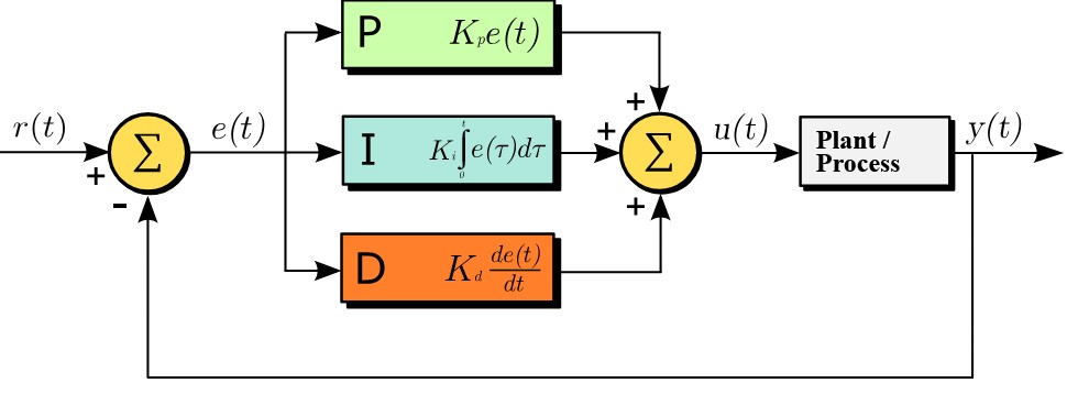 PID Controller
The standard mathematical expression of a PID controller is:
\[u(t) = K_{\text{p}} \left(e(t) + \frac{1}{T_{\text{i}}} \int_{0}^{t} e(\tau)\,\mathrm{d}\tau + T_{\text{d}} \frac{\mathrm{d} e(t)}{\mathrm{d} t} \right)\]Let’s break down this formula into simple terms:
- $u(t)$ is the control output (For example, how much brake apply to the dyno).
- $e(t)$ is the Error (Setpoint (speed we want to reach) - Actual Measurement(current speed)).
We can configure the controller with the following three parameters, Proportional ($K_p$), Integral ($K_i$), and Derivative ($K_d$):
- P (Proportional): This looks at the current error. If you are going 50 RPM and your target is 100 RPM, the error is large, so the controller pushes the throttle hard. As you get closer to 100 RPM, the error is reduced, and the throttle is reduced. P alone usually leaves a small gap (steady-state error) because if the error hits zero, the throttle goes to zero, and the car slows down again.
- I (Integral): This accumulates past errors over time. If the car is stuck at 98 RPM on a hill, the proportional term might not be strong enough to close the gap. The integral term notices this continuous 2 RPM error, adds it up over time, and steadily increases the throttle until you finally reach 100 RPM, your setpoint.
- D (Derivative): This looks at the rate of change of the error. If you are accelerating toward your target RPM very rapidly, the D term anticipates that you might overshoot (go over 100 RPM). It essentially acts as a brake, easing off the throttle to ensure the RPM lands smoothly on the target without oscillating.
Here there are three graphs, on each one I change only one parameter, the first one the Kp, the second one the Ki and the third one the Kd to check how the parameter affects to the system output:
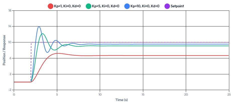 Different Kp Values
We can see how the Kp parameter makes the system react faster or slower to a change. If the value is too high, the system will overshoot and exhibit some oscillations.
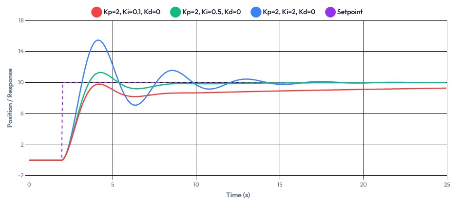 Different Ki Values
With the Ki parameter, we control the accumulation of error over time, as can be seen here.
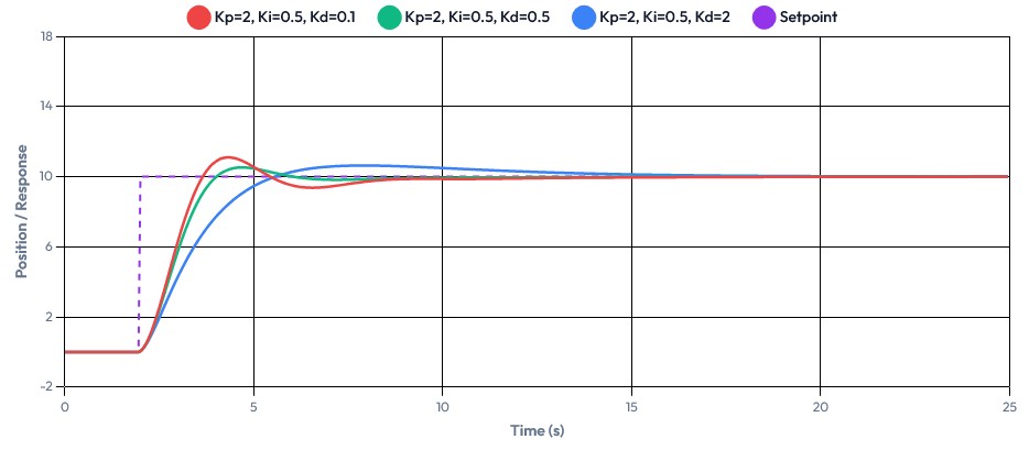 Different Kd Values
Finally, the Kd parameter, which reacts to the rate of change of the error, helps dampen oscillations and improves system stability.
Some systems use only PI control, while others use full PID control. There are multiple configurations, but they are outside the scope of this discussion.
Application to this Project
Knowing that we are going to use a PID controller in this project, we need to clearly define our system variables. As discussed previously, the dynamometer will have three distinct working modes. By breaking these down, we can define the input, output, and control direction for each mode:
Speed Mode
- Setpoint: Target speed, defined by the user (in RPM).
- Input (Feedback): Actual speed, read by the encoder.
- Output: PWM Duty Cycle, sent to the power stage (the eddy current brake).
- Control: Reverse.
Torque Mode
- Setpoint: Target torque, defined by the user (in Nm).
- Input (Feedback): Actual torque, read by the load cell.
- Output: PWM Duty Cycle, sent to the power stage (the eddy current brake).
- Control: Direct.
Acceleration Mode
- Setpoint: Target acceleration, defined by the user (in RPM/s2).
- Input (Feedback): Actual acceleration, calculated from the encoder readings.
- Output: PWM Duty Cycle, sent to the power stage (the eddy current brake).
- Control: Reverse.
Direct vs Reverse Control
Another critical concept we must understand before writing our code is the direction of the control action. Depending on what we are trying to control, applying more power to our actuator (the eddy current brake) will either drive our measured feedback up or down:
-
Direct: In a direct acting system, if the measured feedback is lower than the setpoint, the controller needs to increase its output. For example, if our target torque is 100 Nm and we are only reading 50 Nm, the PID must apply more brake (increase the PWM output) to load the motor heavier and raise the torque. Because we increase the output to increase the reading, this is a direct mode.
-
Reverse: In a reverse acting system, if the measured feedback is lower than the setpoint, the controller must decrease its output. For example, if our target speed is 3000 RPM but the motor is struggling at 2000 RPM, the PID must decrease the braking force (lower the PWM output) to allow the speed to increase. Because we decrease the output to increase the reading, this is a reverse mode.
For this project, I am running the PID loop at 1 kHz (1000 Hz). This means the entire PID calculation, reading the sensor, calculating the error, and updating the output happens every 1 millisecond.
A common mistake in control systems is pairing a high-frequency PID loop with slow sensors or outputs. This is what happened to me in the first try with the thyristor module. For the system to remain stable, the entire control chain must be matched in speed:
- Feedback Frequency: Must update at least as fast as the PID loop.
- Output Update Rate: Must update at least as fast as the PID loop.
In this application, the RPM feedback frequency depends on the actual speed of the shaft. At low RPM, the update rate is naturally slower. However, once the dynamometer reaches its working RPM range, the feedback frequency exceeds the PID loop frequency, ensuring stability.
Regarding the torque measurement, if an HX711 is used for the load cell, the update rate becomes a bottleneck at only 80 Hz. To achieve a more responsive system, using the ADS1220 ADC allows for higher sampling rates.
The PWM output also operates at 1 kHz. This is sufficient for an eddy current brake because the system is not using a fast-discharge capacitor as explained in the DynoPower stage. The high inductance of the brake coils acts as a natural low-pass filter, making the physical response of the system inherently slower than the electrical control signal.
Another common requirement in PID control is that the sampling frequency should be between 5x and 20x higher than the system bandwidth. In this case, a 1 kHz control loop is more than sufficient due to the slow dynamics introduced by the eddy current brake inductance and the mechanical inertia of the system.
QuickPID Library
Before developing my own code, I tried to find a library or existing code with an accurate implementation of a PID Controller. After testing different libraries, the one that I liked more was QuickPID.
The usage is quite simple, let’s use the speedPID as example:
Initialization:
1
2
3
4
5
6
7
8
9
10
11
12
13
14
#include "QuickPID.h"

QuickPID speedPID(
    &status.current_speed,      // Input: Current RPM from encoder
    &status.pid_output,         // Output: PWM control value (0-65535)
    &config.mode.value,         // Setpoint: Target RPM from user
    config.speed_pid.kp,        // Proportional gain
    config.speed_pid.ki,        // Integral gain
    config.speed_pid.kd,        // Derivative gain
    QuickPID::pMode::pOnErrorMeas, // Proportional on Error and Measurement
    QuickPID::dMode::dOnMeas,      // Derivative on Measurement (prevents derivative kick)
    QuickPID::iAwMode::iAwClamp,   // Integral Anti-Windup via clamping
    QuickPID::Action::reverse      // Reverse action (more brake = less speed)
);
Configuration:
1
2
3
4
5
6
7
8
9
10
11
void setup() {
    // Set output limits. Units are PWM percent (0–330 by default);
    // setDutyPercent() converts to 16-bit (0–65535) inside.
    speedPID.SetOutputLimits(0, config.pwm_config.pwm_limit);

    // Set sample time to 1ms
    speedPID.SetSampleTimeUs(1000);

    // Enable the PID controller
    speedPID.SetMode(QuickPID::Control::automatic);
}
Then, on each iteration of the PID:
1
2
3
4
5
6
7
8
9
10
11
void loop() {
    // Standard 1ms task scheduler
    if (pending_1ms) {
        // Step 1: Execute PID calculation
        speedPID.Compute();
        // Step 2: Apply the calculated output through the safety/filter path.
        // set_pwm() clamps to [pwm_start, pwm_limit], applies the output LPF,
        // and finally calls setDutyPercent() which writes the 16-bit PWM register.
        set_pwm(status.pid_output, config, outputFilter, status);
    }
}
With this clarified, we can now go a bit deeper into the modes and options.
Analyzing Working Modes
The QuickPID library provides the flexibility to alter how the proportional, derivative, and integral terms are computed. Below, I analyze these modes for each term.
Proportional Mode
In a PID controller, the proportional term ($P$) provides a control action that is directly proportional to the instantaneous error as seen previously. The library offers three ways to calculate this term:
- Proportional on Error (
pOnError)- $P = K_p \times e$
- This is the classic proportional response, where the output reacts directly to the error ($e = Setpoint - Measurement$). While responsive, a sudden step change in the setpoint instantly creates a massive error, causing a spike in the output known as a proportional kick. This aggressive reaction can lead to system overshoot.
- Proportional on Measurement (
pOnMeas)- $P = -K_p \times \Delta PV$
- Instead of reacting to the error, it reacts to how fast the sensor reading itself is moving ($\Delta PV$). If the input is changing fast, it pushes back. Changing the setpoint does not cause a sudden output spike because the sensor has not moved yet. On the other side, it has a slower response to a new setpoint.
- Proportional on Error and Measurement (
pOnErrorMeas)- $P = 0.5(K_p \times e) - 0.5(K_p \times \Delta PV)$
- This mode acts as a hybrid, splitting the proportional calculus exactly in half between the error and the measurement. It provides a compromise between both modes.
Derivative Mode
The derivative term ($D$) tries to predict future error by looking at the rate of change. The library gives us two choices for calculating the derivative term:
- Derivative on Error (
dOnError)- $D = K_d \times \Delta e$
- This mode reacts to how fast the error is changing. If the error is decreasing quickly, it backs off the output to avoid overshooting. On the other hand, if the setpoint changes fast, the error jumps instantly causing a “derivative kick”.
- Derivative on Measurement (
dOnMeas)- $D = -K_d \times \Delta PV$
- This mode reacts to how fast the sensor reading is changing, not the error. The sensor moves smoothly in the real world, so this avoids the derivative kick when the setpoint changes.
Integral Mode
Understanding Integral Windup The integral term ($I$) accumulates past errors over time to eliminate steady-state offset. Imagine that your system has a huge setpoint change, but the actuator hits its physical limit (for example, the PWM signal is at 100%). While the system tries to catch up, the error persists and the integral term keeps accumulating. This is called windup. When the system finally reaches the target setpoint, this integral accumulation must “unwind” but they are slow due to the accumulated error. Anti-windup strategies try to avoid this.
QuickPID has three integral anti-windup modes:
- Integral Anti-Windup Off (
iAwOff)- No anti-windup protection is applied to the accumulated integral term.
- Integral Anti-Windup Clamp (
iAwClamp)IntegralSum = constrain(IntegralSum, OutputMin, OutputMax)- This applies a bounding approach. When the internal or accumulated integral value tries to exceed the physical limits of your systems output, it is clamped at those limits. It forcefully stops the integral from winding up higher once saturation is reached.
- Integral Anti-Windup Condition (
iAwCondition)- This is the smartest mode. It only activates anti-windup when two conditions are both true. When the projected output is already beyond the limit (saturated) and when the error is still growing in the same direction.
Safety Mechanisms
To handle a software fault, a communication failure, or an invalid configuration that could result in the brake locking up at full power, the firmware implements safety mechanisms to guarantee that the system is always under control.
Bidirectional Heartbeat Watchdog
Both the microcontroller and the server application send periodic heartbeat messages over CAN, and each side monitors the other for liveness.
Server to Microcontroller: The server sends a heartbeat message. When the microcontroller receives it, it resets a watchdog timer and sets status.connected = true. If no valid heartbeat arrives within 4 seconds (SECURITY_CHECK_INTERVAL), the microcontroller assumes the server has crashed, the CAN cable is disconnected, or the application has been closed and declares a disconnected state.
1
2
3
4
5
6
7
8
9
10
11
12
// Receiving a heartbeat (inside parse_can_message):
case APP_HEARTBEAT_ID:
    if (incoming.data[0] == APP_HEARTBEAT_VALUE)
    {
        status.connected = true;
        last_security_time_check = millis(); // Reset watchdog
    }
    else
    {
        status.connected = false; // Invalid value - reject
    }
    break;
1
2
3
4
5
// Watchdog check (every loop iteration):
if (millis() - last_security_time_check > SECURITY_CHECK_INTERVAL)
{
    status.connected = false; // Timeout - no heartbeat received
}
Microcontroller to Server: The microcontroller sends its own heartbeat every 100 ms. The server monitors this to detect if the microcontroller has crashed.
Disconnect Failsafe
When the heartbeat watchdog triggers a disconnected state, the enforce_disconnect_failsafe() function is called on every single loop iteration. It forces a complete safe shutdown:
1
2
3
4
5
6
7
8
9
10
11
12
13
14
15
16
17
18
19
20
21
22
23
24
static void enforce_disconnect_failsafe(void)
{
    if (status.connected)
        return;

    // Force safe state immediately
    status.status = STOPPED;
    status.info = INFO_MSG_STOPPED;
    status.manual_pwm_enabled = false;
    status.pid_output = 0.0f;
    status.pwm_value = 0.0f;

    // Disable all PID controllers
    torquePID.SetMode(QuickPID::Control::manual);
    speedPID.SetMode(QuickPID::Control::manual);
    dynamicPID.SetMode(QuickPID::Control::manual);
    brakeDynamicPID.SetMode(QuickPID::Control::manual);
    speedLimitPID.SetMode(QuickPID::Control::manual);

    // Bypass set_pwm() path - write zero directly to hardware
    outputFilter.y_prev = 0.0f;
    outputFilter.timestamp_prev = 0;
    setDutyPercent(0.0f);
}
This will disable all braking in the dyno.
Configuration Checksum Gate
The PID controllers will not execute unless the configuration has been validated via CRC-16 checksum. The microcontroller computes a CRC-16 over its local Configuration structure and compares it against the checksum sent by the server. Only when both match is status.valid_checksum set to true.
Every PID mode check includes this guard:
1
2
3
4
if (config.mode.mode == SPEED_MODE && status.status == RUNNING && status.valid_checksum)
{
    run_speed_pid();
}
This means the brake will never actuate with corrupted, partially received, or default PID gains. If the server sends a new configuration and the checksums do not match, the system automatically requests a retransmission until integrity is confirmed.
Minimum Speed Cutoff
All PID controllers include a minimum speed threshold (default: 500 RPM). If the measured speed falls below this value, the brake is immediately released. On the other side, the PWM will not actuate until the brake has reached the minimum RPM. This is used to protect the eddy current brake as it is not recommended to power it with high current at low RPM.
1
2
3
4
5
6
7
8
9
10
11
12
13
void run_speed_pid(void)
{
    if (status.current_speed < config.speed_limits.min_speed)
    {
        status.info = INFO_MSG_LOW_SPEED;
        set_pwm(0, config, outputFilter, status); // Release brake
    }
    else
    {
        speedPID.Compute();
        set_pwm(status.pid_output, config, outputFilter, status);
    }
}
Filters
Sensor signals are inherently noisy. Mechanical vibrations, electrical interferences among others contribute to measurement noise. If these raw signals were fed directly into the PID controllers or displayed to the user, the system would oscillate or produce unreadable data.
The system uses four different types of filters, each chosen for a specific purpose and placed at a specific point in the signal chain:
| Filter | Type | Where Used | Purpose |
|---|---|---|---|
| Hardware glitch filter | Silicon (ENC1) | Encoder input | Reject pulses < ≈167 ns |
| Ratio outlier rejector | Non-linear | Encoder period samples | Reject single-sample spikes (period outside 0.526×…1.9× of previous); force-reconverge after 10 rejects |
| Cascaded IIR LPF | 1st-order × N | Speed (1× @ 20 Hz), Torque (4× @ 15 Hz), Acceleration (2× @ 10 Hz) | Continuous noise smoothing |
| Single IIR LPF | 1st-order | PID output (20 Hz) | Smooth PWM command changes |
| Block Average (100 samples) | Linear | Hall current sensor (1 kHz, sync to PWM ON-time) | Oversampling noise reduction |
Low-Pass Filter
This is the primary filter used across all major signals. It is the equivalent of an analog RC low-pass circuit. Its defining characteristic is that it uses a single configurable parameter, the cutoff frequency to control how it smooths the output.
The filter equation is:
\[y_n = \alpha \cdot x_n + (1 - \alpha) \cdot y_{n-1}\]Where the smoothing factor α is computed dynamically from the actual elapsed time between calls:
\[\alpha = \frac{\Delta t}{T_f + \Delta t}, \qquad T_f = \frac{1}{2\pi f_c}\]The implementation code:
1
2
3
4
5
6
7
8
9
10
11
12
13
14
15
16
17
18
19
20
21
float lowPassFilter(float x, float frequency, LowPassFilter &filter)
{
    if (frequency <= 0) return x;

    unsigned long timestamp = micros();

    if (filter.timestamp_prev == 0) filter.timestamp_prev = timestamp;

    float dt = (timestamp - filter.timestamp_prev) * 1e-6f;
    filter.timestamp_prev = timestamp;

    // Sanity check: reject implausible dt values
    if (dt <= 0.0f || dt > 0.5f) dt = 1e-3f;

    float Tf = 1.0f / (6.2831853f * frequency);
    float alpha = dt / (Tf + dt);

    float y = alpha * x + (1.0f - alpha) * filter.y_prev;
    filter.y_prev = y;
    return y;
}
Each filtered signal uses its own filter state instance and a configurable cutoff frequency. The implementation actually cascades N identical first-order stages. Speed uses 1 stage, torque uses 4 stages, and acceleration uses 2 stages. The stage counts are fixed at compile time and the cutoff frequencies are runtime-configurable.
A lower cutoff produces a smoother signal but adds more phase lag, which is exactly the trade-off to watch when tuning the PID.
Block Averaging (Hall Sensor)
The Hall effect current sensor uses oversampling and block averaging to reduce the noise inherent in magnetic current sensing. The system samples the ADC at 1 kHz (synchronized with the PWM “ON” state) and accumulates these into a running sum.
Every 100 ms, the system calculates the average:
1
2
3
4
5
6
7
8
9
10
11
12
13
14
15
16
17
18
19
20
21
22
23
24
25
26
27
28
29
30
struct hall_sensor_averager
{
	volatile float sum;           // Running sum of ADC readings [volts]
	volatile uint16_t count;      // Number of samples in current block
	float last_average;           // Most recent averaged value [volts]

	void reset()
	{
		sum = 0.0f;
		count = 0;
	}

	void add_sample(float voltage)
	{
		sum += voltage;
		count++;
	}

	float compute_average()
	{
		if (count > 0)
		{
			last_average = sum / count;
			reset();
			return last_average;
		}
		return last_average;  // Return previous if no new data
	}
};
typedef struct hall_sensor_averager HallSensorAverager;
With 100 samples per block, this averaging reduces random noise by roughly 10x, providing a stable current reading.
Speed Mode
As described above, speed mode maintains a constant RPM by varying the braking torque. The implementation uses a single QuickPID library controller (speedPID) with the encoder-measured speed as the process variable and the user-defined RPM setpoint as the target.
The PID is configured with reverse action: when the measured speed exceeds the setpoint, the output increases (more braking). When the speed drops below, the output decreases (less braking). This is the inverse of a typical heating controller and reflects the nature of a brake.
1
2
3
4
5
6
7
8
9
10
11
// PID wiring: input = measured speed, output = PWM, setpoint = target RPM
QuickPID speedPID((float *)&status.current_speed,
                  &status.pid_output,
                  &config.mode.value,           // Setpoint from server
                  config.speed_pid.kp,
                  config.speed_pid.ki,
                  config.speed_pid.kd,
                  QuickPID::pMode::pOnErrorMeas, // P on error+measurement (anti-kick)
                  QuickPID::dMode::dOnMeas,      // D on measurement (no derivative kick)
                  QuickPID::iAwMode::iAwClamp,   // Integral anti-windup via clamping
                  QuickPID::Action::reverse);     // Reverse: more speed -> more braking
The execution is straightforward. If the speed is above the minimum threshold, the PID computes and drives the PWM. Otherwise, the brake is released as a safety measure:
1
2
3
4
5
6
7
8
9
10
11
12
13
void run_speed_pid(void)
{
    if (status.current_speed < config.speed_limits.min_speed)
    {
        status.info = INFO_MSG_LOW_SPEED;
        set_pwm(0, config, outputFilter, status);
    }
    else
    {
        speedPID.Compute();
        set_pwm(status.pid_output, config, outputFilter, status);
    }
}
Key implementation choices:
pOnErrorMeas: The proportional term is split between error and measurement. This reduces the proportional kick that would otherwise appear when the setpoint changes. (The derivative kick is addressed separately bydOnMeasbelow.)dOnMeas: The derivative term acts on the measurement, not the error. This prevents a large spike in PID output when the setpoint changes fast.iAwClamp: Integral anti-windup via clamping prevents the integral term from accumulating beyond the output limits, which would cause overshoot when the system transitions between states.
Torque Mode
Torque mode maintains a constant braking torque using load cell feedback. The PID controller (torquePID) uses the measured torque as the process variable and the user-defined Nm setpoint as the target.
Unlike speed mode, this PID uses direct action: when the measured torque is below the setpoint, the output increases (more PWM = more braking = more torque). When the torque exceeds the setpoint, the output decreases.
1
2
3
4
5
6
7
8
9
10
11
// PID wiring: input = measured torque, output = PWM, setpoint = target Nm
QuickPID torquePID((float *)&status.current_torque,
                   &status.pid_output,
                   &config.mode.value,             // Setpoint from server
                   config.torque_pid.kp,
                   config.torque_pid.ki,
                   config.torque_pid.kd,
                   QuickPID::pMode::pOnErrorMeas,
                   QuickPID::dMode::dOnMeas,       // D on measurement
                   QuickPID::iAwMode::iAwClamp,    // Anti-windup
                   QuickPID::Action::direct);      // Direct: more torque needed -> more PWM
The execution follows the same pattern:
1
2
3
4
5
6
7
8
9
10
11
12
13
void run_torque_pid(void)
{
    if (status.current_speed < config.speed_limits.min_speed)
    {
        status.info = INFO_MSG_LOW_SPEED;
        set_pwm(0, config, outputFilter, status);
    }
    else
    {
        torquePID.Compute();
        set_pwm(status.pid_output, config, outputFilter, status);
    }
}
Acceleration Mode
Acceleration mode controls the rate of speed change (RPM/s) using the computed acceleration as the process variable. This mode uses the dynamicPID controller with reverse action: when acceleration exceeds the setpoint, more braking is applied to slow it down. When acceleration drops, braking is reduced to allow faster acceleration.
1
2
3
4
5
6
7
8
9
10
11
// PID wiring: input = measured acceleration, output = PWM, setpoint = target RPM/s
QuickPID dynamicPID((float *)&status.current_acc,
                    &status.pid_output,
                    &config.mode.value,           // Setpoint from server
                    config.dynamic_pid.kp,
                    config.dynamic_pid.ki,
                    config.dynamic_pid.kd,
                    QuickPID::pMode::pOnErrorMeas, // P on error+measurement (anti-kick)
                    QuickPID::dMode::dOnMeas,      // D on measurement (no derivative kick)
                    QuickPID::iAwMode::iAwClamp,   // Anti-windup
                    QuickPID::Action::reverse);     // Reverse: more accel -> more braking
1
2
3
4
5
6
7
8
9
10
11
12
13
void run_acceleration_pid(void)
{
    if (status.current_speed < config.speed_limits.min_speed)
    {
        status.info = INFO_MSG_LOW_SPEED;
        set_pwm(0, config, outputFilter, status);
    }
    else
    {
        dynamicPID.Compute();
        set_pwm(status.pid_output, config, outputFilter, status);
    }
}
This PID uses the same pOnErrorMeas / dOnMeas family as the speed and torque loops. The dedicated deceleration controller (brakeDynamicPID) is the only one that uses pOnMeas instead.
Dynamic Mode
Dynamic mode is the most complex operating mode. It orchestrates a complete acceleration test by automatically transitioning through multiple phases, each using a different PID controller and setpoint. I implemented 8-state state machine.
State Machine Overview
stateDiagram-v2
    [*] --> IDLE
    IDLE --> SPINUP_TO_START_SPEED: Start command

    SPINUP_TO_START_SPEED --> WAIT_STABLE: Speed ≥ start_speed

    WAIT_STABLE --> ACCELERATING: Stable for N ms
    WAIT_STABLE --> WAIT_STABLE: Speed unstable

    ACCELERATING --> HOLD_TOP_SPEED: Speed ≥ end_speed

    HOLD_TOP_SPEED --> WAIT_TORQUE_DROP: Hold timer expired

    WAIT_TORQUE_DROP --> DECELERATING: Torque drop ≥ 15% for 200ms

    DECELERATING --> FINISHED: Speed ≤ final_speed

    FINISHED --> IDLE: Reset
State 1: IDLE
This state is used to prepare the dyno for the test. Also to clean and restart a test after a previous one:
1
2
3
4
5
6
7
case IDLE:
    set_pwm(0, config, outputFilter, status);
    speedLimitPID.SetMode(QuickPID::Control::automatic);
    dynamicPID.SetMode(QuickPID::Control::manual);
    dyno_baseline_valid = false;
    dyno_enter_state(SPINUP_TO_START_SPEED);
    break;
State 2: SPINUP_TO_START_SPEED
The speedLimitPID holds the brake at a level that allows the motor to spin up to the configured start_speed. This stabilizes the torque applied to the dyno to start the dynamic test.
1
2
3
4
5
6
7
8
9
10
11
case SPINUP_TO_START_SPEED:
    limit_speed = config.dynamic_config.start_speed;
    speedLimitPID.Compute();
    set_pwm(status.pid_output, config, outputFilter, status);

    if (status.current_speed >= config.dynamic_config.start_speed)
    {
        dyno_stable_enter_ms = 0;
        dyno_enter_state(WAIT_STABLE);
    }
    break;
State 3: WAIT_STABLE
Before transitioning to the measurement phase, the system waits for the speed to stabilize within +-5 RPM of the start_speed for a configurable duration (stable_time_ms, by default: 2 seconds). If the speed drifts out of tolerance at any point, the timer resets:
1
2
3
4
5
6
7
8
9
10
11
12
13
14
15
16
17
18
19
20
21
22
23
24
case WAIT_STABLE:
    limit_speed = config.dynamic_config.start_speed;
    speedLimitPID.Compute();
    set_pwm(status.pid_output, config, outputFilter, status);

    if (speed_within_tol(status.current_speed,
                         config.dynamic_config.start_speed,
                         static_config.stable_speed_tolerance))
    {
        if (dyno_stable_enter_ms == 0)
            dyno_stable_enter_ms = now;
        else if (now - dyno_stable_enter_ms >= config.dynamic_config.stable_time_ms)
        {
            // Stable long enough - switch to acceleration PID
            speedLimitPID.SetMode(QuickPID::Control::manual);
            dynamicPID.SetMode(QuickPID::Control::automatic);
            dyno_enter_state(ACCELERATING);
        }
    }
    else
    {
        dyno_stable_enter_ms = 0; // Not stable - reset timer
    }
    break;
State 4: ACCELERATING
This is the core measurement phase. The dynamicPID controls the acceleration rate. The system also captures a baseline torque reading on the first positive measurement, which will be used later for torque drop detection:
1
2
3
4
5
6
7
8
9
10
11
12
13
14
15
16
17
18
case ACCELERATING:
    dynamicPID.Compute();
    set_pwm(status.pid_output, config, outputFilter, status);

    // Capture baseline torque for drop detection
    if (!dyno_baseline_valid && status.current_torque > 0.0f)
    {
        dyno_baseline_load = status.current_torque;
        dyno_baseline_valid = true;
    }

    if (status.current_speed >= config.dynamic_config.end_speed)
    {
        dynamicPID.SetMode(QuickPID::Control::manual);
        speedLimitPID.SetMode(QuickPID::Control::automatic);
        dyno_enter_state(HOLD_TOP_SPEED);
    }
    break;
State 5: HOLD_TOP_SPEED
The speed limit PID holds the motor at end_speed for a configurable duration (hold_ms). This acts as a safety motor limit to avoid overspeed.
1
2
3
4
5
6
7
8
case HOLD_TOP_SPEED:
    limit_speed = config.dynamic_config.end_speed;
    speedLimitPID.Compute();
    set_pwm(status.pid_output, config, outputFilter, status);

    if (now - dyno_hold_start_ms >= config.dynamic_config.hold_ms)
        dyno_enter_state(WAIT_TORQUE_DROP);
    break;
State 6: WAIT_TORQUE_DROP
This state waits and detects when the user releases the throttle. It computes a smoothed relative torque drop against the captured baseline. The smoothing (30% new, 70% old) prevents false triggers from measurement noise. The drop must persist for 200 ms to be confirmed:
1
2
3
4
5
6
7
8
9
10
11
12
13
14
15
16
17
18
19
20
21
22
23
24
25
26
case WAIT_TORQUE_DROP:
{
    static float last_load = 0.0f;
    static uint32_t drop_detected_ms = 0;

    // Smooth torque reading
    last_load = (last_load * 0.7f) + (status.current_torque * 0.3f);

    // Calculate relative drop from baseline
    float rel_drop = 0.0f;
    if (dyno_baseline_load > 0.0f)
        rel_drop = (dyno_baseline_load - last_load) / dyno_baseline_load;

    // Require 15% drop sustained for 200 ms
    if (rel_drop >= static_config.torque_drop_threshold)
    {
        if (drop_detected_ms == 0) drop_detected_ms = now;
        else if (now - drop_detected_ms >= 200)
            dyno_enter_state(DECELERATING);
    }
    else
    {
        drop_detected_ms = 0; // Reset - insufficient drop
    }
}
break;
State 7: DECELERATING
A dedicated brakeDynamicPID controller applies a controlled deceleration at the configured rate (accel_down). The setpoint is negative to indicate braking.
1
2
3
4
5
6
7
8
9
10
11
12
13
14
case DECELERATING:
    dynamic_brake = -fabsf(config.dynamic_config.accel_down);
    brakeDynamicPID.SetMode(QuickPID::Control::automatic);
    brakeDynamicPID.Compute();
    set_pwm(status.pid_output, config, outputFilter, status);

    if (status.current_speed <= config.dynamic_config.final_speed)
    {
        brakeDynamicPID.SetMode(QuickPID::Control::manual);
        set_pwm(0, config, outputFilter, status);
        status.status = STOPPED;
        dyno_enter_state(FINISHED);
    }
    break;
State 8: FINISHED
The test is complete. The state machine resets to IDLE, the brake is released, and the system status is set to STOPPED.
State Transition Notifications
Every state change calls dyno_enter_state(), which updates the status.info field and immediately sends a CAN status broadcast. This allows DynoServer to display the current test phase in real time:
1
2
3
4
5
6
7
8
9
10
11
12
13
14
15
16
17
18
static void dyno_enter_state(dynamic_dyno_state s)
{
    dyno_state = s;

    switch (s)
    {
        case IDLE:                  status.info = INFO_MSG_IDLE; break;
        case SPINUP_TO_START_SPEED: status.info = INFO_MSG_SPINUP; break;
        case WAIT_STABLE:           status.info = INFO_MSG_WAIT_STABLE; break;
        case ACCELERATING:          status.info = INFO_MSG_ACCELERATING; break;
        case HOLD_TOP_SPEED:        status.info = INFO_MSG_HOLD_TOP_SPEED; break;
        case WAIT_TORQUE_DROP:      status.info = INFO_MSG_WAIT_TORQUE_DROP; break;
        case DECELERATING:          status.info = INFO_MSG_DECELERATING; break;
        case FINISHED:              status.info = INFO_MSG_FINISHED; break;
    }

    send_can_status(status); // Notify server immediately
}
PIDs used on each state
The dynamic mode switches PID controllers at each transition always disabling the outgoing controller before enabling the incoming one.
| Test State | Active Controller | Type |
|---|---|---|
IDLE |
speedLimitPID |
Speed Mode |
SPINUP_TO_START_SPEED |
speedLimitPID |
Speed Mode |
WAIT_STABLE |
speedLimitPID |
Speed Mode |
ACCELERATING |
dynamicPID |
Dynamic Mode |
HOLD_TOP_SPEED |
speedLimitPID |
Speed Mode |
WAIT_TORQUE_DROP |
speedLimitPID |
Speed Mode |
DECELERATING |
brakeDynamicPID |
Dynamic Mode |
FINISHED |
All PIDs OFF | None |
DynoServer
With the firmware running on the microcontroller, it is time to address the server side. This section is divided into two main parts: frontend and backend. The frontend covers everything related to the graphical interface and user interaction with the web application, while the backend addresses the details behind the server.
For this project I chose Flask for the backend since I had some experience programming with this Python Framework. For the frontend, as we will see below, I used the Bootstrap library and JavaScript for the dynamic elements of the web page.
I am aware that modern frameworks like Next.js or React exist, but I did not use any of them because I had no experience with them and because when I started the project I thought it would be simpler and that I would not need anything like that.
Technology Stack
| Layer | Technology | Purpose |
|---|---|---|
| Backend | Flask (Python) | HTTP server, REST API, Template Rendering |
| Real-time | Flask-SocketIO and Eventlet | WebSocket bidirectional communication |
| CAN Interface | python-can | CAN bus communication with microcontroller |
| Frontend | Bootstrap 5 + Bootstrap Icons | Frontend Components |
| Charts | uPlot and ApexCharts | High-performance real-time charting |
| Interactivity | jQuery + JavaScript | DOM manipulation, UI Logic |
| Data Storage | JSON files | Persistent Configuration |
Project Structure
1
2
3
4
5
6
7
8
9
10
11
12
13
14
15
16
17
18
19
20
21
22
23
24
25
26
27
28
29
30
31
DynoServer/
├── run.py                       # Application entry point
├── config/
│   └── __init__.py              # Environment-based Flask configuration
├── app/
│   ├── __init__.py              # Flask application factory + SocketIO init
│   ├── api/
│   │   └── routes.py            # REST API endpoints
│   ├── web/
│   │   └── views.py             # HTML page routes
│   └── services/
│       ├── can_manager.py       # CAN bus communication
│       ├── can_commands.py      # CAN message definitions
│       ├── can_ids.py           # CAN Message IDs
│       ├── config_manager.py    # Configuration persistence + CRC16 calculation
│       ├── data_manager.py      # Test logs Operations
│       └── input_validation.py  # Request payload validation
├── templates/
│   ├── base.html                # Base template
│   ├── index.html               # Main dashboard
│   ├── configuration.html       # Full configuration page
│   ├── debug.html               # Debug page
│   └── logs.html                # Saved test log viewer
├── static/
│   ├── css/                     # Bootstrap + custom stylesheets
│   └── js/
│       ├── app/                 # Application JavaScript
│       └── vendor/              # Bootstrap, jQuery, Popper, uPlot
└── data/
    ├── config.json              # Runtime configuration
    └── database.json            # Saved test logs
Backend
The server uses Flask’s application factory pattern (create_app()). This function:
- Creates the Flask application with template and static folder paths
- Loads environment configuration
- Initializes Flask-SocketIO with Eventlet as the async mode
- Registers two blueprints:
web_app(Frontend Pages) andapi(REST Endpoints) - Creates the core service instances (
ConfigManager,CANManager) - Starts the CAN listener thread and calculates an initial configuration checksum
- Registers WebSocket event handlers and a shutdown cleanup handler
1
2
3
4
5
6
7
8
9
10
11
12
13
14
15
16
17
18
19
20
21
22
def create_app(config_name=None):
    app = Flask(__name__,
                template_folder=os.path.join(base_dir, '..', 'templates'),
                static_folder=os.path.join(base_dir, '..', 'static'))

    config_obj = get_config(config_name)
    app.config.from_object(config_obj)

    socketio.init_app(app, cors_allowed_origins=app.config['ALLOWED_ORIGINS'])

    # Register route blueprints
    app.register_blueprint(web_app)
    app.register_blueprint(api)

    # Initialize and wire up services
    config_manager = ConfigManager(app.config['CONFIG_PATH'], system_manager)
    can_manager = CANManager(socketio, system_manager, app.config)
    system_manager.set_config_manager(config_manager)
    system_manager.set_can_manager(can_manager)

    can_manager.start_listener()
    return app
Blueprints and Routing
Flask Blueprints are used to organize routes into logical modules:
Web App Blueprint: Serves HTML pages:
| Route | Template | Description |
|---|---|---|
/ |
index.html |
Main dashboard |
/config |
configuration.html |
System configuration |
/debug |
debug.html |
Debug page with PID tuning charts |
/logs |
logs.html |
Saved test log analyzer |
API Blueprint: REST API with /api prefix:
| Endpoint | Method | Purpose |
|---|---|---|
/api/run |
GET | Send START command to microcontroller |
/api/stop |
GET | Send STOP command to microcontroller |
/api/tare |
GET | Calibrate the load cell |
/api/update_live |
POST | Enable/disable live data streaming |
/api/update_pwm |
POST | Set manual PWM value |
/api/config |
GET | Get full configuration |
/api/config |
POST | Update full configuration |
/api/fastConfig |
GET | Get reduced config |
/api/fastConfig |
POST | Update reduced config |
/api/logs |
GET | List all saved test logs |
/api/logs |
POST | Save a new test log |
/api/logs/<id> |
GET | Get specific test log by ID |
/api/logs/<id> |
DELETE | Delete test log by ID |
/api/status |
GET | Get current system status |
All POST endpoints validate their payloads through input_validation.py before processing, returning structured JSON errors if validation fails.
CAN Manager (3 Threads)
The CANManager manages the physical CAN bus interface and runs three concurrent daemon threads:
-
Listener thread: Continuously calls
bus.recv(timeout=1.0)and dispatches incoming messages. -
Periodic sender: Sends the application heartbeat every 500 ms and the configuration checksum every 1000 ms.
-
Watchdog: Checks every 500 ms whether a heartbeat from the microcontroller has been received within the last 2 seconds. If not, it marks the connection as lost and notifies all browser clients.
Data Unpacking
Incoming CAN messages are unpacked using Python’s struct module, mirroring the firmware’s little-endian packing format:
1
2
3
4
5
6
7
8
9
10
11
12
import struct
# Speed: little-endian uint16, 0.1 RPM resolution
brake_speed_rpm = struct.unpack_from('<H', payload, 0)[0] / 10

# Torque: little-endian uint16, 0.01 kg resolution
current_torque_kg = struct.unpack_from('<H', payload, 2)[0] / 100.0

# Timestamp: little-endian uint32
timestamp_ms = struct.unpack_from('<I', payload, 4)[0]

# Temperature: little-endian float (raw IEEE 754)
brake_temp = struct.unpack('<f', bytes(msg.data))[0]
Gear Ratio Conversion
All values from the microcontroller are measured at the brake side. The server converts them to motor side values using the configured pinion ratio before sending to the browser:
1
2
3
# Motor side conversion using pinion ratios
motor_speed = brake_speed_rpm * dyno_pinions / motor_pinions
motor_torque_nm = brake_torque_nm * motor_pinions / dyno_pinions
This conversion is applied in _parse_live_data(), which is shared between the filtered and debug live data handlers.
Inertia Compensation
Because the dynamometer has rotating inertia, the measured torque at the brake is not the true motor torque during acceleration. The server adds an inertial-torque correction. The acceleration is measured in the firmware (filtered, then transmitted on CAN 0x09); the server converts it to rad/s2, multiplies by the brake-side inertia, and then scales that inertial torque back to the motor side using the pinion ratio:
1
2
3
4
5
6
# can_manager._parse_live_data()
alpha_brake          = (acceleration_filtered * 2 * math.pi) / 60.0       # RPM/s -> rad/s2
total_brake_inertia  = dyno_inertia + chain_inertia                       # kg x m2
inertia_torque_brake = total_brake_inertia * alpha_brake                  # Nm at the brake
inertia_torque_motor = inertia_torque_brake * (motor_pinions / dyno_pinions)
motor_torque_comp_nm = motor_torque_nm + inertia_torque_motor             # Nm at the motor
The browser-side live_data payload therefore carries four torque fields: brake_torque (raw load-cell), motor_torque (gear-scaled, uncompensated), inertia_torque (the J·α correction), and torque (the compensated motor torque, used for plotting and power). This ensures the torque curve displayed in the charts reflects the motor’s output, not just the braking force.
Power is not computed in the firmware or the server. The browser computes it from the filtered torque and speed it receives:
1
const power_kW = (filteredTorque_Nm * filteredSpeed_rpm * 2 * Math.PI) / 60 / 1000;
Configuration Manager and Checksum
The ConfigManager handles configuration persistence (JSON file) and the CRC-16 checksum calculation that ensures DynoServer (Python) and DynoLogic (C) synchronization.
CRC-16 Checksum Calculation
The checksum must be identical on both sides, in the Python server and the C firmware. To achieve this, the server packs the JSON configuration into a binary struct that matches the exact memory layout of the firmware’s Configuration struct, including padding and alignment:
1
2
3
4
5
6
7
8
9
10
11
12
13
14
15
16
17
18
19
20
21
def calculate_crc16(self, config_dict):
    expected_size = 108  # sizeof(Configuration) on ARM Cortex-M7
    data = bytearray(expected_size)
    offset = 0

    # debug_mode (uint8_t) + 3 bytes padding -> bytes 0..3
    struct.pack_into('<B', data, offset, 1 if config_dict.get("debug", {}).get("enabled") else 0)
    offset += 4

    # torque_pid (3 floats) -> bytes 4..15
    torque = config_dict.get("torquePID", {})
    struct.pack_into('<fff', data, offset,
                     float(torque.get("kp", 0)),
                     float(torque.get("ki", 0)),
                     float(torque.get("kd", 0)))
    offset += 12

    # ... speed_pid, dynamic_pid, run_mode, load_cell, pwm, filters, limits, dynamic_config
    # Each field is packed in the exact same order and alignment as the C struct

    return self.crc16(data)
The CRC-16 algorithm:
1
2
3
4
5
6
7
8
9
10
def crc16(self, data: bytes) -> int:
    crc = 0xFFFF
    for b in data:
        crc ^= b
        for _ in range(8):
            if crc & 1:
                crc = (crc >> 1) ^ 0xA001
            else:
                crc >>= 1
    return crc
The checksum is recalculated and sent to the microcontroller every second by the periodic sender thread. If the DynoLogic computed CRC does not match, it requests a full configuration from the DynoServer.
Frontend
The frontend runs in the browser of the user. It is the part of the application responsible of showing a smooth data and allow the user to manage the dynamometer.
WebSockets
All real-time data flows through WebSockets using Socket.IO. The browser opens a WebSocket connection on page load:
1
const socket = io({ transports: ['websocket'] });
The server emits events whenever CAN data arrives, and the browser listens for specific event types:
1
2
3
4
socket.on('env', function (data) {
    updateDOMText('env_temperature', data.temperature + " °C");
    updateDOMText('env_humidity', data.humidity + " %");
});
Real-Time Charts (uPlot)
The charting library used is uPlot. After testing different libraries like Apache eCharts and others, uPlot was the fastest, best-performing library I found. Data is updated every 10 ms.
Display-side filtering: Independently of the firmware filters, the browser applies its own smoothing purely for the on-screen chart and number cards: a 5-sample moving average on speed, and a 2-stage IIR low-pass filter (2 Hz cutoff, 100 Hz sample rate) on torque. A toggle in the Graph Configuration modal lets the user switch this display filter off. Crucially, when the user saves a test log, the RAW (un-filtered) samples are stored.
New data points are appended to arrays incrementally rather than re-rendering the entire dataset. When the buffer exceeds the configured maximum points (by default 500), the oldest points are shifted out. The user can configure the number of points that the chart can plot. This improves the performance of the chart rendering:
1
2
3
4
5
6
7
8
9
10
11
12
13
14
15
socket.on('live_data', function(data) {
    timestamps.push(data.timestamp / 1000);  // ms -> seconds
    speedData.push(data.motor_speed);
    torqueData.push(data.torque);
    powerData.push(data.torque * data.motor_speed * 2 * Math.PI / 60 / 1000);

    if (timestamps.length > maxPoints) {
        timestamps.shift();
        speedData.shift();
        torqueData.shift();
        powerData.shift();
    }

    chart.setData([timestamps, speedData, torqueData, powerData]);
});
Gear Ratio Conversion (Motor - Brake)
The user always sees motor values (RPM, Nm), but the microcontroller operates in brake values. The frontend converts in both directions using the configured pinion ratio:
1
2
3
4
5
6
7
// Motor - Brake (when saving to server)
brakeSpeed = motorSpeed * motorPinions / dynoPinions;
brakeTorque = motorTorque * dynoPinions / motorPinions;

// Brake - Motor (when displaying to user)
motorSpeed = brakeSpeed * dynoPinions / motorPinions;
motorTorque = brakeTorque * motorPinions / dynoPinions;
Other details
There are few details that need to be improved:
This application has two different measurement domains: brake and motor. All the data measured and calculated by the firmware is from the eddy current brake. This is correct, but the user wants to know the power, speed and torque of the tested motor. Because the motor and the dynamometer are linked via a chain ratio (motor pinions vs brake pinions), a mathematical conversion must occur between these two domains.
Imagine a scenario where you configure a speed mode, setting a specific motor RPM:
- Target Motor Speed: 3000 RPM
- Gear Ratio: 14 / 43 (Motor Pinions / Brake Pinions)
When the frontend prepares to send this configuration to the DynoLogic, it calculates the equivalent targeted in brake speed:
Brake RPM = 3000 * (14 / 43) = 976.744186... RPM
If the configuration system only saves integer data, it rounds this math off: 977 RPM. This value will be sent over CAN so integer conversion is needed.
The issue arises the next time you open the web interface and it loads that configuration back from the config.json file. To display the stored settings on the dashboard, the UI must reverse the math:
Motor RPM = 977 * (43 / 14) = 3000.785... RPM
Because of the decimals lost during rounding, you would no longer see the 3000 RPM originally entered. Instead, the input shows 3001 RPM.
To ensure the firmware gets the correct value while preserving the user input value, the system saves these variables as a pair inside the config.json:
1
2
3
4
5
"runMode": {
  "mode": 1,
  "value": 977,
  "rawValue": 976.7441860465116
}
When the frontend loads the configuration, it ignores the rounded value for display purposes. Instead, it loads the rawValue to perform the reverse calculation:
Motor RPM = 976.7441860465116 * (43 / 14) = 3000.00 RPM
Of course this is not the best option so I will fix it in the future.
Communication Protocol
In the DynoLogic - CAN-Bus section I explained the entire physical (hardware) implementation of the CAN Bus. In this section we will focus on the logical side.
Within the CAN standard, there are several versions. One of them is CAN 2.0A, also known as Standard CAN, which uses 11-bit identifiers allowing up to 2048 unique message IDs.
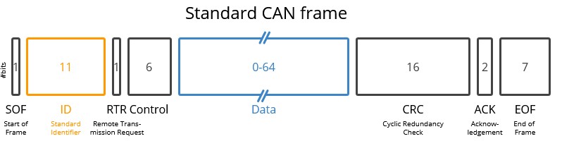 CAN Frame
The most important part for us is the ID and Data sections. The ID will set the receiver of the CAN Frame and the data will be the payload transmitted. We can send up to 8 bytes in one CAN Frame.
I used this variant, running at a bus speed of 500 kbps through the Teensy 4.1’s built-in CAN1 peripheral (ACAN_T4::can1) on the firmware side, and the python-can library via a USB-CAN adapter (slcan0 interface) on the server side.
For that I used a CANable USB interface connected to the Raspberry Pi. With this setup ready, let’s dive into the protocol.
Message ID Architecture
The protocol divides the ID space into two non-overlapping ranges to clearly distinguish the direction of communication and prevent confusion.
- Microcontroller to Server
- Server to Microcontroller
Here you have a complete table of all the commands and instructions that the protocol implements:
Microcontroller to Server
These are the telemetry and status messages sent by the DynoLogic to the DynoServer. Each message has a specific transmission rate and data format.
0x01 - Live Speed & Torque
This message sends the current speed of the eddy current brake and the torque with it’s timestamp.
- Rate: 100 Hz (10 ms)
- Data length: 8 bytes
- Function:
send_speed_torque_timestamp()
| Bytes | Type | Field | Resolution |
|---|---|---|---|
| 0-1 | uint16_t |
Speed (filtered) | 0.1 RPM |
| 2-3 | uint16_t |
Torque (filtered) | 0.01 kg |
| 4-7 | uint32_t |
Timestamp | Miliseconds |
0x02 - System Status
It sends the current status of the system.
- Rate: 2 Hz (500 ms)
- Data length: 8 bytes
- Function:
send_can_status()
| Byte | Type | Field | Description |
|---|---|---|---|
| 0 | uint8 |
Connected | 0 = disconnected, 1 = connected |
| 1 | uint8 |
System Status | 0x00 = STOPPED, 0x01 = RUNNING, 0x02 = DEBUG |
| 2 | uint8 |
Info Code | Status/sub-state code |
| 3 | uint8 |
Live Mode | 0 = disabled, 1 = enabled |
| 4-5 | uint16_t |
PWM Value | Current PWM output |
| 6-7 | uint16_t |
Config Checksum | Local CRC16 of Configuration struct |
0x03 - Configuration Request
This message is sent by the microcontroller when it starts up or the checksum is invalid. The DynoServer should answer with all the configuration of the system.
- Rate: On-demand
- Data length: 1 byte
- Function:
send_configuration_request()
| Byte | Type | Field | Value |
|---|---|---|---|
| 0 | uint8 |
Request | 0x01 (CONFIG_REQUEST_BYTE) |
0x04 - Electrical Current
This message sends the current applied to the eddy current brake.
- Rate: 10 Hz (100 ms)
- Data length: 8 bytes
- Function:
send_electrical_data()
| Bytes | Type | Field | Unit |
|---|---|---|---|
| 0-3 | float |
Current | Amps |
| 4-7 | uint32_t |
Timestamp | ms since boot |
0x05 - Electrical Voltage
This message sends the voltage applied to the eddy current brake.
- Rate: 10 Hz (100 ms)
- Data length: 8 bytes
- Function:
send_electrical_data()
| Bytes | Type | Field | Unit |
|---|---|---|---|
| 0-3 | uint32_t |
Voltage | millivolts |
| 4-7 | uint32_t |
Timestamp | ms since boot |
0x06 - Microcontroller Heartbeat
This message is sent by the microcontroller to let the DynoServer know that it’s still alive. If this message is not sent (or received by DynoServer) it will think that the DynoLogic board is shut down or disconnected.
- Rate: 10 Hz (100 ms)
- Data length: 1 byte
- Function:
send_heartbeat()
| Byte | Type | Field | Value |
|---|---|---|---|
| 0 | uint8 |
Heartbeat | 0x20 (MICRO_HEARTBEAT_VALUE) |
0x07 - Environmental Data (BME280)
This message sends the environmental temperature and humidity read by the BME280 sensor.
- Rate: 0.2 Hz (5 s)
- Data length: 8 bytes
- Function:
send_env()
| Bytes | Type | Field | Unit |
|---|---|---|---|
| 0-3 | uint32_t |
Temperature | °C (integer) |
| 4-7 | uint32_t |
Humidity | % (integer) |
0x08 - PID Debug Data
- Rate: 100 Hz (10 ms)
- Data length: 8 bytes
- Function:
send_pid_debug_data()
| Bytes | Type | Field | Notes |
|---|---|---|---|
| 0-1 | uint16_t |
Setpoint | Rounded from config.mode.value |
| 2-3 | uint16_t |
PWM Value | Scaled × 100 |
| 4-7 | uint32_t |
Timestamp | ms since boot |
0x09 - Filtered Acceleration
- Rate: 100 Hz (10 ms)
- Data length: 6 bytes
- Function:
send_acceleration_timestamp()
| Bytes | Type | Field | Unit |
|---|---|---|---|
| 0-1 | int16_t |
Acceleration (filtered) | RPM/s |
| 2-5 | uint32_t |
Timestamp | ms since boot |
0x10 - Brake Temperature (MLX90614)
- Rate: 1 Hz (1 s)
- Data length: 4 bytes
- Function:
send_brake_temperature()
| Bytes | Type | Field | Unit |
|---|---|---|---|
| 0-3 | float |
Temperature | °C |
0x11 - Raw Acceleration (Debug)
- Rate: 100 Hz (10 ms)
- Data length: 6 bytes
- Function:
send_acceleration_debug_timestamp()
| Bytes | Type | Field | Unit |
|---|---|---|---|
| 0-1 | int16_t |
Acceleration (raw) | RPM/s |
| 2-5 | uint32_t |
Timestamp | ms since boot |
0x12 - Raw Speed & Torque (Debug)
- Rate: 100 Hz (10 ms)
- Data length: 8 bytes
- Function:
send_speed_torque_debug_timestamp()
| Bytes | Type | Field | Resolution |
|---|---|---|---|
| 0-1 | uint16_t |
Speed (raw) | 0.1 RPM |
| 2-3 | uint16_t |
Torque (raw) | 0.01 kg |
| 4-7 | uint32_t |
Timestamp | ms since boot |
0x13 - Ambient Temperature (DS18B20)
- Rate: 1 Hz (1 s)
- Data length: 4 bytes
- Function:
send_ds18b20_temperature()
| Bytes | Type | Field | Unit |
|---|---|---|---|
| 0-3 | float |
Temperature | °C |
Server to Microcontroller
0x100 - Operation Mode Configuration
- Sender:
send_run_config() - Data length: 3 bytes
| Byte | Type | Field | Values |
|---|---|---|---|
| 0 | uint8 |
Mode | 0 = Torque, 1 = Speed, 2 = Dynamic, 3 = Acceleration |
| 1-2 | uint16_t |
Setpoint | Target RPM / Nm / RPM/s |
0x101 - Start / Stop Command
- Sender:
send_start()/send_stop() - Data length: 1 byte
| Byte | Type | Field | Value |
|---|---|---|---|
| 0 | uint8 |
Command | 0x00 = STOP, 0x01 = START |
0x102 - Server Heartbeat
- Sender: Periodic thread (500 ms)
- Data length: 1 byte
| Byte | Type | Field | Value |
|---|---|---|---|
| 0 | uint8 |
Heartbeat | 0x10 (APP_HEARTBEAT_VALUE) |
0x103 - Configuration Checksum (CRC16)
- Sender: Periodic thread (1000 ms)
- Data length: 2 bytes
| Bytes | Type | Field |
|---|---|---|
| 0-1 | uint16_t |
CRC16 of 108-byte Configuration struct |
0x104 - Debug Mode Toggle
- Sender:
send_debug_config() - Data length: 1 byte
| Byte | Type | Field | Value |
|---|---|---|---|
| 0 | uint8 |
Debug Mode | 0 = disabled, 1 = enabled |
0x105 - Live Data Streaming Toggle
- Sender:
set_live() - Data length: 1 byte
| Byte | Type | Field | Value |
|---|---|---|---|
| 0 | uint8 |
Live Mode | 0 = disabled, 1 = enabled |
0x106 - Manual PWM Override
- Sender:
set_pwm_value() - Data length: 2 bytes
| Bytes | Type | Field | Notes |
|---|---|---|---|
| 0-1 | int16_t |
PWM Value | Only accepted when STOPPED |
0x107 - Load Cell Tare
- Sender:
tare_load_cell() - Data length: 1 byte
| Byte | Type | Field | Value |
|---|---|---|---|
| 0 | uint8 |
Tare Command | 0x00 triggers tare |
0x109-0x111 - Torque PID Gains
- Sender:
send_torque_pid_config() - Data length: 4 bytes each (float)
| CAN ID | Field |
|---|---|
0x109 |
Torque Kp |
0x110 |
Torque Ki |
0x111 |
Torque Kd |
0x112-0x114 - Speed PID Gains
- Sender:
send_speed_pid_config() - Data length: 4 bytes each (float)
| CAN ID | Field |
|---|---|
0x112 |
Speed Kp |
0x113 |
Speed Ki |
0x114 |
Speed Kd |
0x115-0x117 - Dynamic PID Gains
- Sender:
send_dynamic_pid_config() - Data length: 4 bytes each (float)
| CAN ID | Field |
|---|---|
0x115 |
Dynamic Kp |
0x116 |
Dynamic Ki |
0x117 |
Dynamic Kd |
0x118 - Load Cell Gain & Offset
- Sender:
send_load_cell_config() - Data length: 4 bytes
| Bytes | Type | Field | Notes |
|---|---|---|---|
| 0-1 | uint16_t |
Gain | HX711 gain (128 or 64) |
| 2-3 | 2 bytes | Padding | Padding |
| 4-7 | float |
Offset | Zero-offset from tare |
0x119 - PWM Configuration
- Sender:
send_pwm_config() - Data length: 6 bytes
| Bytes | Type | Field | Notes |
|---|---|---|---|
| 0-1 | uint16_t |
PWM Start | Minimum duty cycle |
| 2-3 | uint16_t |
PWM Limit | Maximum duty cycle |
| 4-5 | uint16_t |
PWM Frequency | Hz (typically 1000) |
0x120 - Low-Pass Filter Configuration
- Sender:
send_low_pass_filters() - Data length: 8 bytes
| Bytes | Type | Field | Unit |
|---|---|---|---|
| 0-1 | uint16_t |
Speed filter cutoff | Hz |
| 2-3 | uint16_t |
Torque filter cutoff | Hz |
| 4-5 | uint16_t |
Acceleration filter cutoff | Hz |
| 6-7 | uint16_t |
PID output filter cutoff | Hz |
0x121 - Speed Safety Limits
- Sender:
send_speed_limits() - Data length: 4 bytes
| Bytes | Type | Field | Unit |
|---|---|---|---|
| 0-1 | uint16_t |
Min Speed | RPM |
| 2-3 | uint16_t |
Max Speed | RPM |
0x122 - Dynamic Config: Start Speed & Stable Time
- Sender:
send_dynamic_config() - Data length: 8 bytes
| Bytes | Type | Field | Unit |
|---|---|---|---|
| 0-3 | float |
Start Speed | RPM |
| 4-7 | float |
Stable Time | ms |
0x123 - Dynamic Config: Ramp Rate & End Speed
- Data length: 8 bytes
| Bytes | Type | Field | Unit |
|---|---|---|---|
| 0-3 | float |
Acceleration Rate | RPM/s |
| 4-7 | float |
End Speed | RPM |
0x124 - Dynamic Config: Hold Time & Deceleration
- Data length: 8 bytes
| Bytes | Type | Field | Unit |
|---|---|---|---|
| 0-3 | float |
Hold Delay | ms at peak speed |
| 4-7 | float |
Ramp Down Rate | RPM/s |
0x125 - Dynamic Config: Final Speed
- Data length: 4 bytes
| Bytes | Type | Field | Unit |
|---|---|---|---|
| 0-3 | float |
Final Speed | RPM |
0x126 - Load Cell Scale & Lever Arm Distance
- Sender:
send_load_cell_config() - Data length: 8 bytes
| Bytes | Type | Field | Unit |
|---|---|---|---|
| 0-3 | float |
Scale | ADC-to-grams factor |
| 4-7 | float |
Distance | Lever arm length (m) |
Final Result 📈
Dynamic Mode
Speed Mode
Torque Mode
Acceleration Mode
Future work
- Current control PI
- Cascade PIDs
- Relay in DynoPower
- CAN Connection to DynoPower
- Speed Implementation (kmh, mph)
- Multiple Eddy Current Brake and Encoder support
- Track mode
Gallery 📷
Mechanical ⚙️
Hardware ⚡
Software 💻
Conclusion
When I started this project, I thought I could finish it in about two months. Over a year later, I can confidently say I was wrong. What began as a simple dynamometer build turned into a deep dive across mechanical design, power electronics, embedded firmware, and full-stack web development. Each discipline brought its own set of unexpected challenges.
The iterative nature of hardware design was one of the hardest lessons. Designing a PCB is not like writing software; you cannot just fix a bug and recompile. Each mistake meant waiting weeks for a new board to arrive, diagnosing the issue, and then starting another revision.
From the slow thyristor module in DynoPower v1, to discovering that SiC MOSFETs were burning out because the gate drive voltage was 12V instead of 15V, to the counterfeit CAN transceivers that wasted days of debugging, every iteration taught me something that no textbook could. The DynoLogic board alone went through multiple revisions, initially built around an Atmel SAM3X8E that became too expensive and had I2C compatibility issues, before migrating to the Teensy 4.1, which offered far better performance at a lower cost.
I also learned that in engineering, the order matters. Fix problems at the mechanical level first, then hardware, then software. I spent weeks trying to filter noisy sensor readings in firmware, only to discover that a stretched chain was the root cause of the vibrations. No amount of software filtering can compensate for a faulty mechanical component.
To my knowledge, this is the only open-source project that provides a complete system for controlling eddy current brake dynamometers, from the power stage and logic board schematics, through the real-time firmware and PID control, to the web-based user interface. While commercial alternatives exist from companies like Perek, none of them offer full visibility into their signal processing, filtering, or data calculation methods. Transparency matters in dynamometry because it is remarkably easy to smooth or manipulate results.
The project is not perfect. There are still unfinished features like the fast discharge circuit, the cascade PID architecture, track simulation mode or the fact that the project is focused on motor dynamometers, not roller ones. The DynoLogic v2 has known hardware bugs that are being addressed. But even in its current state, the system works and produces repeatable, reliable test results.
Commercial Alternatives
This project is Open Source, and while it offers a solid foundation, there are still many features to develop and issues to resolve. If you are looking to build a professional grade dynamometer, several companies specialize in high-end electronics:
- Perek6: In my opinion, this company offers the most advanced electronics on the market. Their PID controls are exceptionally well-implemented, featuring high-frequency power stages and robust fast discharge circuits for precise brake control. Their documentation is comprehensive, and I recommend them without hesitation. One of their biggest strengths is that they focus on dynamometer electronics, allowing them to specialize deeply in features that truly matter for accuracy.
- SportDevices: This company manufactures both complete dynamometers and standalone electronics. While they offer a fast discharge version, it may not be as sophisticated as Perek’s implementation. It is worth noting that some designs rely more heavily on resistive dissipation rather than capacitive energy absorption for field collapse, which can affect response times during rapid load changes.
- YourDyno: YourDyno focuses primarily on the electronics and software ecosystem. While some users find their hardware interface a bit more traditional compared to the latest other designs, the system is highly reliable and features very frequent software updates. It is a proven solution that works well for both DIY enthusiasts and professional workshops.
There are many other companies in the market, but the most critical factor to consider is transparency. You should choose a provider that is open about how signals are processed, which filters are applied, and how the final data is calculated. In the world of dynamometers, it is easy to smooth or manipulate results. Accuracy and data integrity should always be your top priorities, but it’s also the hardest part to develop.
References: